A Selective Profiling Tool: Towards Automatic Performance Tuning Abhinav Bhatele1 , and Guojing Cong2 1
University of Illinois at Urbana-Champaign Dept. of Computer Science Urbana, IL 61801-2302 USA
[email protected]
Abstract We present some preliminary results of selective profiling in our efforts towards automatic performance tuning for scientific codes. Performance analysis and tuning are becoming very important with the increasing complexity and speed of high performance systems. Great efforts are necessary to tune applications for optimal performance on such systems. In our efforts to automate most, if not all, of the performance tuning process, we have developed a flexible profiling tool that can quickly pinpoint the performance bottlenecks and further refine the problem area. This is an important first step in our open framework with a rule-based approach for the ongoing PERCS project.
1. Introduction High performance computing (HPC) is essential in advancing science and society. In recent years, HPC systems such as Blue Gene [1] are becoming increasingly powerful and complex. Tremendous human efforts are necessary in tuning an application for optimal performance on these systems. It would greatly increase the productivity of performance engineers if, the bulk of the tuning process could be automated. Currently it still remains more or less a philosophical question whether without human input, a performance problem can be identified automatically by a computer itself. However, from observing the most effective engineers working on performance optimizations in an industrial laboratory, we are convinced that in many scenarios the applications can be automatically tuned for the target arc 1-4244-0910-1/07/$20.00 2007 IEEE.
IBM Research Thomas J. Watson Research Center Yorktown Heights, NY 10598 USA
[email protected] 2
chitectures. One such approach is for each scenario to define and apply the corresponding transformation that eliminates the performance bottleneck. The pool of scenarios and transformations may not be exhaustive, but we expect to catch most of the everyday recurring problems. Note that this is a large project and we have barely begun our research in this area. The current approach may not be the best as it involves more heuristic than systematic ways for tackling this problem. We present the development of our flexible profiling tool under this context. There are currently plenty of software tools, some of which are very powerful and if properly used can help pinpoint hard-to-find performance bottlenecks and/or correctness issues. However, for the tuning of scientific codes on usually dedicated HPC systems, these tools may be too complex to use, and after much effort the user might still be left with a huge list of choices, unsure of which transformation to use to best improve the performance. We have had the opportunity to observe the process or steps that many performance engineers take with their applications and platforms, and have noticed that many performance problems and their solutions are highly repetitive in different applications. In our efforts to design performance support tools under the PERCS project for the DARPA HPCS program [4], we strive to determine the transformations that are sure to help boost performance. Profiling is invariably the first step that an engineer takes when he is faced with the task of determining the bottlenecks and tuning an application. Profiling gives a rough idea of how much time each program construct (usually on the statement or function level) takes to execute. After identifying the most time consuming constructs, the engineer can then further collect more performance information and investigate whether there is any mismatch between the program and the architecture that causes performance degrada-
3. Our Profiling Tool
tion. In this paper we present our implementation of a profiling tool that is flexible and facilitates these efforts. This is our first step in automating the performance tuning process. Some of the best features in this tool which are important but non-existent in the current profiling tools are: it does not need to access the source code nor does it need recompilation for profiling. However, we believe its value lies more in its contribution to automatic performance tuning. The rest of the paper is organized as follows: Section 2 presents a brief review of the profiling technique and current profiling tools. Section 3 and 4 describe the design and implementation of our profiling tool. Section 5 compares our implementation with other existing profiling tools; Section 6 discusses the work in progress and finally Section 7 is the conclusion and future work.
We have developed a new profiling tool that is capable of selectively profiling an arbitrary set of routines. The tool on one hand implements the functionality provided by gprof and on the other hand, provides means to further narrow down to the bottlenecks. The implementation is based on binary rewriting. Binary rewriting has been used in studying the behavior of the application for optimization purposes [3]. We observe that augmenting an application for profiling is a perfect case of application of binary rewriting. Binary rewriting obviates the need for access to the source code, and avoids recompiling the code with the profiling options. We found that similar ideas to tamper with either the binary or the process have been explored independently by other researchers (for example, see [7]). In [7], however, the profiling only works for very simple applications and gives wrong results for commonplace programs like gzip. It does not work for MPI applications either. In addition to an efficient, correct implementation and extensive comparison with gprof , our contribution lies more in the selective approach for program analyis. We present selective profiling in Section 6. As a first step, we have designed our tool to be compatible with gprof . Our tool is to be as efficient as gprof , and the profiling data produced by our tool can also be processed by gprof . The data format adopted by gprof does not always accommodate the information we would like to store. Our tool also produces data in a different format that is more conducive to automatic tuning. Here we give a detailed description of our implementation based on binary rewriting to simulate gprof .
2. Brief Review of Profiling Profiling is the standard technique for studying the behavior of large, complex programs. As current applications are routinely composed of millions of lines of codes, the ability to quickly pinpoint regions that take up most of the execution time is critical to performance tuning. The classical approach involves compiler-generated monitoring routines for the collection of control flow information and sampling for an estimate of the time distribution over the program address space. The first and possibly the most commonly used profiler is gprof [8]. It is able to present counts of routine invocations and timing information for statements. There are two parts to profiling a program with gprof : 1. augment the code at “strategic” points for measuring routine calls and statement executions, 2. sample the value of the program counter at some intervals, and infer execution time from the distribution of the samples within the program. The profiler gprof is not to be confused with the post processing command gprof provided for post processing on most UNIX systems. There are a variety of similar tools that differ in minor implementation details, for example, tprof [10] and jprof [5]. gprof is probably the most frequently used tool by performance engineers. While very useful, gprof has some restricting limitations, especially in the context of automatic performance tuning. For instance, access to the source code and recompilation are necessary for inserting profiling routines. The source codes are often proprietary to a vendor and recompiling complex programs can take a painstakingly long time especially when a high optimization level is used. Also gprof does not differentiate between code regions. As a result, performance metrics at the same level of detail are collected across the whole program and most of them do not bring insights into detecting the performance problem. A profiling tool that is flexible and leads towards automatic performance tuning is thus highly desirable.
4. Sampling and Call Graph Generation For statistical approximation of the execution time for each statement, gprof samples the program counter (PC) value regularly. Sampling does not necessarily require special support from the operating system. On most versions of Unix and alike systems, sampling can be naturally supported by time slicing. On dedicated systems, like the operating system for Blue Gene where time sharing and multiprogramming are not supported, user managed timer interrupts can be used. The interface to the sampling utility is in general the profil(buffer, bufsize, lowpc, scale) routine that registers a buffer to record the clock ticks that occur inside a range of addresses. Choosing appropriate parameter values, we can achieve the effects such as higher precision for a shorter range of addresses. gprof counts the number of times each routine is invoked as well as the arc (parent/children relationship) in the call graph that activated the profiled routine. The compiler generated monitoring routine (usually mcount) is immediately
2
called by each profiled routine and the monitoring routine’s return address is recorded. Obviously this address falls inside the profiled routine that is the destination of an arc in the call graph. The monitoring routine also identifies the call site or the source of the arc. There can be millions, even up to billions of dynamic function calls during an execution. gprof maintains a hash table of all arcs discovered, using the call site address as the primary key and the callee address as the secondary key. A linked list is used to resolve the conflicts into the hash table entry. We employ similar data structures and algorithms as in gprof .
is calculated by a simple divide on the caller’s address. So the hash function used is trivial to calculate and collisions occur only for call sites that call multiple destinations (e.g. functional parameters and functional variables). The hash table is implemented using arrays. We have an array for the caller functions and another for storing the callee functions’ address and the count. The data structure is output to a file at the end of the program. Blindly intercepting each function call with graphgen can cause unexpected behavior. Infinite recursive invocation to a function occurs if it is also called by graphgen. For example, if function f1 is intercepted with graphgen and f1 is in turn called from within graphgen, there will be an infinite sequence of graphgen → f1 → graphgen → f1 → . . . For most functions this generally would not occur as they are not called by graphgen. For those function calls to system libraries inside graphgen, for example memset, our solution is to provide our own version of implementation that is guaranteed not to appear elsewhere. Binary instrumentation can also cause problems with another patched-in routine which is called initialize. This routine is patched in before the entry into the first user function because it initializes the data structures used for storing the profiling information. In this routine, we use malloc to allocate memory for the hash table and other data structures. The call to malloc will be intercepted by graphgen to record the caller/callee arc if it is used by the user program. Consider the execution of a binary augmented for profiling. We will observe the following sequence of function calls supposing the binary is compiled from a C program that calls malloc: main → initialize → malloc → graphgen → . . . Notice that at the time graphgen is called, the memory for the hash table is not yet allocated because we are intercepting the call to malloc for allocating the memory for profiling. Our solution is to have a piece of static array for the initial table. Anyway as this table grows dynamically during the lifespan of the execution, reallocation is to be performed.
4.1. Sampling In order to simulate gprof , we start profiling once the program control first enters user code and stop it just before we write out the collected data to the output file. We thus need to detect the entry and exit of user code, and patch in the profil routine. Detecting the entry is quite simple with most of the binary formats like ELF [2] and XCOFF [11]. To ensure the stopping of sampling, we register a request to stop the execution of profil at the exit of a program using the atexit utility. For this a call to profil(NULL, 0, 0, 0) is patched in. All the information obtained from profiling is stored in a buffer whose pointer is passed on to the profil routine initially. Once the program ends, this buffer is written to the output file.
4.2. Call Graph Generation Our implementation of the monitoring routine is slightly different from mcount as the patching involves “jumps” using trampolines that do not constitute full function calls, hence the stack walking should be treated differently. The monitoring routine we have implemented is called graphgen and is patched in at the entry of every function. The basic algorithm we use for recording call graph information is similar to what is used by gprof . We go over it here briefly. When a function call is made, a counter is incremented for the particular caller-callee arc. The method of obtaining the caller and callee address have been discussed above. One can not afford to have the monitoring routine output tracing information as each arc is identified. Therefore, the monitoring routine maintains a data strucure in the memory, of all the arcs discovered with counts of the number of times each is traversed during execution. This structure is accessed once per routine call. Access to it must be as fast as possible so as not to overwhelm the time required to execute the program. The solution is to use a hash table. We use the call site as the primary key with the callee address being the secondary key. Since each call site typically calls only one callee, we can reduce the number of minor lookups (usually to one) based on the callee. The hash
4.3. Binary Patching We instrument the binary and patch in the monitoring routine graphgen for each function. That is, we modify the binary so that at the entry of each function, a call to graphgen is issued. The graphgen routine walks the stack and registers the call site and callee in the hash table. The entry of the first user function (for example, main) is intercepted for initialization and setting up the profiling environment. The initialize function is patched in for this purpose. At exit, we patch in the function which outputs the sampling data and the call graph, to a binary file called “gmon.out”. We use the SIGMA [6] tool for binary rewriting on AIX.
3
Figure 1. Call graph constructed from the profiling data collected by gprof . The figure on the left is a global clustered view of the entire call graph. The part on the right shows a zoomed in view of the orphan cluster on the bottom right.
from this library are not visible to our instrumentation. For example, for gzip about 20 extra function calls from libc are profiled in the compiler generated code for to get a total of 63 functions. Our implementation instruments in total around 40 functions that we can detect from the symbol table. For most applications, the execution inside libc is very seldom of concern. The relative ranking of the user functions is usually more informative. We are able to profile function calls to precompiled libraries that gprof fails to capture the caller-callee relationship for. If the identity of the caller of a function cannot be determined, the caller is labeled as “spontaneous”. This can happen for signal handlers. Function calls to precompiled libraries that were not augmented by the compiler for profiling will result in many “spontaneous” callers. Although the execution time for each individual function is still captured, the call graph is broken into many distinct components. This can be a problem if a significant amount of time is spent inside the precompiled library, for example, the communication library, I/O library, and other highly optimized math libraries. We test our implementation with SKaMPI [9]. The SKaMPI benchmark is a suite of tests designed to measure the performance of Message Passing Interface (MPI) implementations. SKaMPI maintains a database to illustrate the performance of machine-dependent MPI implementations. The majority of the code is on MPI communications. On AIX, the profiling library of the POE environment is not provided. Figure 1 is the graphical presentation of a profiled run with collective communication primitives. On the left we present a clustered view of the call graph as there are too
4.4. Output and Post Analysis The output file is called “gmon.out” as in gprof and shares the same format. Eventually the profiling data is output for post-analysis when the program terminates. We have customized an in-house post processing tool Xprofiler for presenting the profiling data. Xprofiler visualizes the call graph using a graphical interface. The routines are represented as boxes while the arcs represent the caller-callee relationship. Xprofiler is also capable of automatically laying out the graph on the screen. We use Xprofiler as it is intuitive and helps the navigation among numerous function calls and arcs.
5. Tests and Results We have done extensive testing of the tool with the SPEC2000 benchmark for correctness and performance. SPEC2000 consists of 12 integer and 14 floating point benchmarks, among which 18 are written in C, 6 in FORTRAN and one each in FORTRAN90 and C++. They range from swim and applu to gzip, gcc and equake, and are good test cases for our implementation. We compare our tool with gprof on AIX. We observed negligible difference for most benchmarks between the execution time of binaries augmented by gprof and our tool. However, it is hard to make a strict comparison between the two as they do not always profile the same set of functions. Current gprof implementation on AIX links against a special profiled library libc where the monitoring routine is precompiled. Some of the functions being called
4
Figure 2. Call graph constructed from the profiling data collected by our tool. The figure at the top is a part of the call graph showing calls to MPI functions. The figure below it is a zoomed in view of the box at the top.
5
References
many functions calls to show individually. The nodes are clustered by the libraries. The arcs between two clusters indicate function invocations. If you look at the third level of the graph, there is a cluster in the right cluster that does not have an ancestor. All the MPI collective communication functions are inside this cluster. gprof does not capture the caller-callee relationship for them. On the right is a partial zoomed in view of the cluster. Figure 2 is the graphical presentation of the profiling data collected by our tool. In the top figure, we show the part of the call tree that contains all the callers of the MPI functions. Below it is a zoomed in view of the part inside the box in the left diagram. We can see that the MPI function calls are no longer dangling in the call tree. They are correctly plugged into the call graph.
[1] F. Allen and G. Almasi. A vision for protein science using a petaflop supercomputer. IBM Systems Journal, 21(40):310– 327, 2001. [2] Tool Interface Standards, ELF: Executable and Linkable Format. ftp://ftp.intel.com/pub/tis, 1998. [3] A. Eustace and A. Srivastava. ATOM: A flexible interface for building high performance program analysis tools. 1994. [4] High productivity computer systems. http://highproductivity.org, 2005. [5] Jprof: Java Glossary. http://mindprod.com/jgloss/jprof.html, 1999. [6] L. DeRose, K. Ekanadham, J. K. Hollingsworth and S. Sbaraglia. Sigma: A simulator infrastructure to guide memory analysis. pages 1–13, 2002. [7] K. C. Lee and H. Lin. Gprof via binary instrumentation using dyninst. 2005. [8] S. L. Graham, P. B. Kessler and M. K. McKusick. Gprof: A call graph execution profiler. ACM SIGPLAN notices, pages 49–57, 1982. [9] SKaMPI Benchmark. http://liinwww.ira.uka.de/∼skampi. [10] Tprof. http://perfinsp.sourceforge.net/tpof.html. [11] IBM XCOFF object file format. http://publib16.boulder.ibm.com/peries/en US/files/aixfiles/ XCOFF.htm.
6. Selective Profiling Quite naturally, our profiling tool has the flexibility of profiling an arbitrary set of functions since our implementation is based on binary rewriting. We can first do a top level profiling of the entire program and then selectively profile the functions that we are interested in for better efficiency. This capability can be very helpful for long-running complex applications on massively parallel systems. The profiling actions taken at function entries and exits may also extend beyond call chain chasing. Various other performance metrics such as timing and hardware event counts can be collected. It would be interesting to add the ability to profile basic blocks/individual statements.
7. Conclusion and Future Work We have developed a profiling tool that patches a binary and does not need access to the source code. As a result, profiling with our tool does not need recompilation. It also has the capability of profiling precompiled libraries. This capability is crucial in analyzing the performance of applications that rely heavily on standard libraries such as math or communication libraries. Our tool also has the flexibility of selectively profiling an arbitrary set of functions with arbitrary actions. We consider this as a new step towards more accurate and useful profiling for performance tuning. In the future, we will further improve the tool for the foundation towards automatic performance analysis and tuning. In the current implementation, when gprof attributes times from a child to different parents, it does it in the ratio of the number of times the child is called by each parent. But we would like to attribute actual times to the parents because it is possible that when the same function is called with different arguments by different functions, it takes different amounts of time to execute. Selective profiling discussed in the previous section will be our primary focus.
6