A Similarity-Based Classification Framework For ...

JOURNAL OF LATEX CLASS FILES, VOL. 6, NO. 1, JANUARY 2007

1

A Similarity-Based Classification Framework For Multiple-Instance Learning Yanshan Xiao, Bo Liu, Zhifeng Hao, and Longbing Cao

Abstract—Multiple-instance learning (MIL) is a generalization of supervised learning which attempts to learn useful information from bags of instances. In MIL, the true labels of instances in positive bags are not available for training. This leads to a critical challenge, namely, handling the instances of which the labels are ambiguous (ambiguous instances). To deal with these ambiguous instances, we propose a novel MIL approach, called SMILE (Similarity-based Multiple-Instance LEarning). Instead of eliminating a number of ambiguous instances in positive bags from training the classifier, as done in some previous MIL works, SMILE explicitly deals with the ambiguous instances by considering their similarity to the positive class and the negative class. Specifically, a subset of instances is selected out from positive bags as the positive candidates and the remaining ambiguous instances are associated with two similarity weights, representing the similarity to the positive class and the negative class, respectively. The ambiguous instances, together with their similarity weights, are thereafter incorporated into the learning phase to build an extended SVM-based predictive classifier. A heuristic framework is employed to update the positive candidates and the similarity weights for refining the classification boundary. Experiments on real-world datasets show that SMILE demonstrates highly competitive classification accuracy and shows less sensitivity to labeling noise than the existing MIL methods. Index Terms—Multiple-Instance Learning, Classification

I. I NTRODUCTION Multiple-instance learning (MIL) [1], [2], [3] is proposed to address the classification of bags, which has been successfully applied in a wide variety of real-world applications, ranging from drug activity prediction [4], [5], [6], image retrieval [7], [8], [9] and natural scene classification [10], [11] to text categorization [12], [13]. In MIL, the labels in the training set are associated with sets of instances, which are called bags. A bag is labeled positive if at least one of its instances is positive; the bag is labeled negative if all of its instances are negative. The task of MIL is to classify unknown bags by using the information from labeled bags. In contrast to standard supervised learning, the key challenge of MIL is that the label of any single instance in a positive bag can be unavailable [14], [15], [16], [17], since a positive bag may contain negative instances in addition to one or more positive instances. The true labels for the instances in a positive bag may or may not be the same as the corresponding bag label, which results in inherent ambiguity of instance labels in positive bags. We call the instances with ambiguous labels ambiguous instances. Yanshan Xiao and Zhifeng Hao are with the School of Computers, Guangdong University of Technology, Guangzhou 510006, China. (email: [email protected]; [email protected]) Bo Liu is with the School of Automation, Guangdong University of Technology, Guangzhou 510006, China. (email: [email protected]) Longbing Cao is with the UTS Advanced Analytics Institute, University of Technology, Sydney, NSW 2007, Australia. (email: [email protected])

To handle the MIL ambiguity problem, different supervised methods have been proposed over the years. Since labels of instances in positive bags are not available, a straightforward approach is to transform the MIL into a standard supervised learning problem by labeling all instances in positive bags as positive [18]. However, these MIL methods are based on the assumption that the positive bags consist of fairly rich positive instances. Moreover, mislabeling the negative instances in positive bags as positive may limit the discriminative power of the MIL classifier. To account for this drawback, another group of MIL methods [12], [19], [20], [21], [22] focuses on selecting a subset of instances from positive bags to learn the classifier. The remaining, unselected instances in positive bags are excluded from the learning phase. For example, RW-SVM [20] designs an instance selection mechanism to select one instance from each positive bag. Together with the negative instances from negative bags, these selected instances are used to build the classifier. EM-DD [21] chooses one instance which is most consistent with the current hypothesis in each positive bag to predict an unknown bag. However, the discriminative ability of these approaches may be restricted. This is because only a subset of instances is used to learn the classifier, while a significant number of remaining instances which may contribute an improvement to the MIL accuracy, is not sufficiently utilized in learning the classifier. In this paper, we propose a novel multi-instance learning method, termed as Similarity-based Multiple-Instance LEarning (SMILE). Instead of excluding a number of ambiguous instances from training the classifier, SMILE explicitly deals with the ambiguous instances by considering their similarity to both the positive class and the negative class. Specifically, we select one instance from each positive bag as the initial positive candidate. Based on the positive candidates, each instance is associated with two similarity weights which represent the similarity to the positive class and the negative class, respectively. These ambiguous instances, together with their similarity weights, are incorporated into an extended formulation of support vector machine (SVM). Based on a heuristic learning framework (see Section IV-D), the selection of positive candidates and similarity weights can be updated to refine the classification boundary. The main contributions of our work are as follows. • We propose a learning framework which converts a MIL problem into a supervised learning problem by considering the similarity of ambiguous instances to the classes. The incorporation of ambiguous instances enables a more powerful classifier with better discriminative ability. • We put forward a novel scheme to measure the similarity of ambiguous instances to the classes. By being associated with the similarity weights, ambiguous instances can


be effectively incorporated in training the classifier. We present an extended formulation of SVM to construct the MIL classifier. Compared to SVM, the extended SVM can incorporate the ambiguous instances, as well as their similarity weights, into the optimization process. • We evaluate our approach on real-world datasets. In the experiments, our approach demonstrates highly competitive classification accuracy and shows less sensitivity to the labeling noise than the existing MIL methods. The rest of this paper is organized as follows. Section II reviews the related work. Section III presents a similaritybased data model and gives an overview of the proposed approach. Section IV gives the details of our approach for binary class classification. Section V extends our approach to multi-class classification by implementing some minor modifications. Experiments are conducted in Section VI. Section VII concludes the paper and outlines the future work. •

II. R ELATED W ORK The proposed SMILE method is an SVM-based MIL approach. In this section, we will review the previous works on MIL and then introduce the basic idea of standard SVM. A. Multi-Instance Learning The initial MIL algorithms are presented in [1], [23], [24], which are based on hypothesis classes consisting of axisaligned rectangles. Then, many MIL methods from different perspectives have been proposed [25], [26], [27], [28], [29]. The first category of works sets the instance labels in positive bags as positive, and a standard supervised learning method or an iterative framework is adopted to train the classifier. For example, Ray and Craven [18] label all the instances in positive bags as positive and standard SVM is used to train the classifier straightforwardly. However, this method relies on the positive bags being fairly rich in positive instances. mi-SVM [12] initializes all instances in positive bags as positive and trains an SVM classifier iteratively until each positive bag has at least one instance classified to be positive. Clearly, mi-SVM focuses on obtaining 100% training accuracy of positive bags. However, if labeling noise exists in positive bags, the accuracy of mi-SVM may be greatly reduced. In MILBoost [30], all instances initially get the same label as the bag label and then a boosting framework is adopted to learn the classifier. However, MILBoost is based on the framework of boosting and may sometimes be less robust [31]. The second category of works [32], [33] designs mechanisms to map a bag of instances into a “bag-level” training vector. Typical examples include DD-SVM [32] and MILES [33]. DD-SVM learns a number of instance prototypes and utilizes them to map every bag to a point. In MILES, the bags are embedded in a new feature space and 1-norm SVM is applied to select the important features (instances) for prediction. However, DD-SVM and MILES may transform the MIL problem into a high dimensionality problem. The dimension of “bag-level” vectors is dependent on the number of training instances. If the instance number is large, the “bag-level” vector may turn out to be extremely high dimensional. To solve

2

this problem, MILIS [34] proposes to select one instance from each positive bag to produce the instance prototypes so that the dimension of “bag-level” vectors can be largely reduced. However, the MIL classification accuracy may be biased since a large number of unselected instances in positive bags cannot be sufficiently utilized in learning the prototypes. The third category of works [19], [21], [22], [20], [33] focuses on selecting a subset of instances from positive bags to learn the classifier. For example, EM-DD [21] chooses one instance which is most consistent with the current hypothesis in each positive bag to predict an unknown bag. MI-SVM [12] adopts an iterative framework to learn an SVM classifier. At each iteration, one instance from each positive bag is selected. Together with the instances in negative bags, the selected instances are used to learn the classifier. RW-SVM [20] selects one instance from each positive bag to train the classifier. However, the discriminative ability of these approaches may be restricted. This is because only a subset of instances in positive bags is used to build the classifier, while a large number of ambiguous instances, which may contribute to the prediction, cannot be properly exploited in learning the classifier. Other methods are also proposed to improve MIL classification accuracy [35], [36], [37], [38]. For example, MissSVM [35] considers the MIL problem as a semi-supervised learning problem, and Citation-kNN [39] extends the K-nearest neighbor method to solve the MIL problem. In this paper, we propose a similarity-based multipleinstance learning method. Compared to the works in the third category, we explicitly utilize the ambiguous instances, which are not sufficiently considered in those works, to learn the MIL classifier. The incorporation of ambiguous instances makes our classifier more discriminative in classifying the positive and negative bags and meanwhile leads to better robustness. B. Support Vector Machine (SVM) Let {(x1 , y1 ), (x2 , y2 ), . . . , (xn , yn )} be a training set, where yi ∈ {+1, −1} and n is the number of instances in the training set. To make the instances more linearly separable, a nonlinear mapping function φ(.) is used to map the data from the input space into a feature space z. The goal of SVM [40] is to find an optimized plane wT φ(x) + b = 0.

(1)

To obtain the optimized plane in (1), we need to solve the following objective function: min F (w, b, ξ) =

n X 1 T w w+c ξi , 2 i=1

yi (wT φ(xi ) + b) ≥ 1 − ξi , ξi ≥ 0,

i = 1, . . . , n

(2)

where ξi are error terms and c is a regularized parameter. We can obtain w and b by resolving problem (2). A test instance φ(x) is classified to the positive class if wT φ(x)+b ≥ 0 holds. Otherwise, it is predicted as negative. In standard SVM (2), an instance is considered in only one class. However, in this paper, the ambiguous instance is considered in different classes and thus associated with


3

more than one similarity weight. Standard SVM cannot handle multiple weights for one instance. To solve this problem, we present an extended formulation of SVM, which can effectively incorporate multiple similarity weights of ambiguous instances into the optimization procedure. III. S IMILARITY-BASED DATA M ODEL AND A LGORITHM OVERVIEW A. Similarity-Based Data Model We first introduce notations to describe the MIL problem. + + − − Let D = {(B1+ , Y1+ ), . . . , (BN + , YN + ), (B1 , Y1 ), . . . , − − (BN − , YN − )} denotes a set of training bags, where Bi+ represents a positive bag with a positive label Yi+ = +1; Bi− denotes a negative bag with a negative label Yi− = −1. N + and N − are the numbers of positive bags and negative bags, respectively. In the following, we will omit the +/- sign when there is no need for disambiguation. Each bag contains a set of instances. The j th instance in + + − + Bi and Bi− is denoted as Bij and Bij , respectively. Bij is + − − associated with a label yij and Bij is with yij . Based on the description of MIL, each positive bag has at least one positive instance and all instances in negative bags are negative. Hence, each positive bag has at least one instance of which the label + − is yij = +1, and it has yij = −1 for all instances in negative bags. The purpose of MIL is to learn a classifier on the training data and use the classifier to predict a new bag. For the sake of convenience, we line up the instances in all bags together, and re-index the instances as {(xi , yi )}. Hence, the training set is transformed into D = {(x1 , y1 ), (x2 , y2 ), . . . , (xi , yi ), . . . , (xl , yl )} (i = 1, 2, . . . , l), where l is the total number of instances in the training bags. We then convert each instance xi (i = 1, . . . , l) to a similarity-based data model which is defined as follows: {x, m+ (x), m− (x)}, +

(3)

−

where m (x) and m (x) represent the similarity of x to the positive class and the negative class, respectively, and it has 0 ≤ m+ (x) ≤ 1 and 0 ≤ m− (x) ≤ 1. Using the similarity-based data model presented in (3), we can convert a multi-instance learning problem into a single-instance learning problem, and the supervised learning methods can be extended to solve the MIL problems. More importantly, by introducing the similarity-based data model, the ambiguous instance, which is usually neglected in the training phase due to its ambiguity nature [12], can be modelled and thereafter included in the learning phase, so that the classifier can be refined to be more discriminative. B. The Overview of SMILE Approach In this section, we provide an overview of our proposed approach according to the similarity-based data model. The proposed approach works in four steps, as illustrated in Fig. 1, where each block indicates an object to be operated on and each arrow denotes an operation performed on the object. Let S + and S − contain the instances from positive bags and negative bags, respectively. The first step is initial positive candidate selection. A subset of instances from positive bags is

selected as initial positive candidates. The subset S + is thereafter separated into two subsets Sp and Sa , i.e., S + = Sp ∪Sa . Sp includes the selected positive candidates from positive bags; Sa contains the remaining, unselected instances from positive bags. The second step is similarity weight generation. The similarity weights are assigned to the training instances. For the instances in S − , m− (x) = 1 and m+ (x) = 0 are set. In terms of the instances in Sp , we let m+ (x) = 1 and m− (x) = 0. For the instances in Sa , we assign two similarity weights, i.e., m+ (x) and m− (x), with 0 < m+ (x) < 1 and 0 < m− (x) < 1. The third step is MIL classifier training. An extended formulation of SVM, termed as similarity-based support vector machine (SSVM), is put forward to learn a MIL classifier based on the presented data model. The last step is positive candidate updating. A heuristic framework is proposed to reselect the positive candidates and update the SSVM classifier until the termination criterion is met. In the testing phase, a new bag B is predicted as positive if at least one instance is classified to be positive by the SSVM classifier. Otherwise, it is predicted as negative. The detail of SMILE approach will be discussed in Section IV and its deployment into multi-class classification will be presented in Section V. To simplify the presentation, we let S ∗− = Sa ∪ S − in the following. IV. T HE SMILE A PPROACH A. Initial Positive Candidate Selection Each positive bag contains at least one positive instance, and it is possible to initially select one instance from the positive bag. This selected instance (called the initial positive candidate) is more likely to be positive, compared to the other instances in the same bag. In this paper, we select the initial positive candidate by modelling the distributions of instances in positive bags and negative bags. In this way, one instance is selected as the initial positive candidate from each positive bag and is then put into the subset Sp . Specifically, the selection of initial positive candidates is based on the following definitions: Definition 1 (Single Set-Based Similarity): Given an instance x and a subset S, the similarity of x to S is defined as R(x, S) =

1 X −||x−xi ||2 e , |S|

(4)

xi ∈S

where R(x, S) represents the similarity of x to the subset S; |S| denotes the subset size of S. It has ||x − xi ||2 = x · x − 2x · xi + xi · xi , where x · xi represents the inner product of x and xi . When a nonlinear mapping function φ(·) is used to map the instance x into the feature space, ||x − xi ||2 in (4) is replaced by ||φ(x) − φ(xi )||2 and we have ||φ(x) − φ(xi )||2 = φ(x) · φ(x) − 2φ(x) · φ(xi ) + φ(xi ) · φ(xi ). In Definition 1, the single set-based similarity R(x, S) is de2 fined based on the exponential decay function, i.e., e−||x−xi || . By using the exponential decay function, the value of R(x, S) falls into the range between 0 and 1. When x lies closer to S, the value of R(x, S) tends to be larger. When x is infinitely far away from the instances in S, it has R(x, S) ≈ 0. The farther


4

Training bags

U pdate positive candidates

{

Fig. 1.

+

+

-

-

B 1 ,......, B N , B 1 ,......, B N

} Select initial positive candidates Separate the training set into 3 subsets: Sp, Sa , S+

-

Generate similarity w eights

x in S x in S x in S -

p

a

(x (x (x

, 1 , 0 ) , m + (x ) , m - (x ) ) , 0 , 1 )

Train SV M classifier SV M M odel: f ( x) = wx i + b

The overview of our proposed approach.

x is from S, the lower the similarity of x to S is, which is consistent with our intuitive observations. Definition 2 (Binary Set-Based Similarity): Given an instance x, subsets S + and S − , the similarity of x to S + is defined as: 1 Q(x ∈ S + |S + ∪ S − ) = [R(x, S + ) + 1 − R(x, S − )], (5) 2 where S + and S − are subsets containing the training instances from positive bags and negative bags, respectively. It can be seen that Definition 2 extends Definition 1 to binary class classification in which the positive class and the negative class are available. In Definition 1, we give a general measurement of similarity between an instance and a subset. Based on Definition 1, we propose a binary set-based similarity measurement in Definition 2, where the positive class and the negative class are both considered in measuring the similarity. In Equation (5), R(x, S + ) is the similarity of x to S + . When the value of R(x, S + ) is larger, it indicates that x is more similar to S + . R(x, S − ) represents the similarity of x to S − , and 1−R(x, S − ) can be considered as the dissimilarity of x to S − . When the value of 1 − R(x, S − ) is larger, x is less similar to S − . Moreover, Q(x ∈ S + |S + ∪S − ) is the average of R(x, S + ) and 1−R(x, S − ). When the instance x lies closer to S + and farther from S − , the value of Q(x ∈ S + |S − ) becomes larger. That is to say, x is more similar to a positive instance and is less likely to be negative. We can also extend Definition 1 to multi-class classification problems where more than two classes are available, as presented in Section V-A. Definition 3 (Positive Candidate): For the positive bag Bi+ (i = 1, . . . , N + ), an instance x is selected as the initial positive candidate, if it satisfies max Q(x ∈ S + |S + ∪ S − ). (6) x∈Bi+

Similar to MILD [22], one instance is selected out from each positive bag as the positive candidate. Intuitively, for any instance in a positive bag, the instance which is most similar to instances in positive bags and has least similarity to those in negative bags, is more likely to be positive compared to the remaining instances in the same bag. Therefore, the instance with maximum value of Q(x ∈ S + |S + ∪ S − ) (6) is chosen to

be the positive candidate. After the positive candidates have been determined, we can further divide S + into two subsets Sp and Sa . Sp contains the positive candidates, while Sa includes the remaining, unselected instances, whose labels are relatively ambiguous compared to the positive candidates. B. Similarity Weight Generation The main task of this step is to generate similarity weights for each ambiguous instance to the positive class and the negative class, respectively. Based on the similarity-based data model, the training set can be transformed into a pseudo dataset which consists of three parts: {x, 1, 0} for the positive candidates in Sp , {x, 0, 1} for the negative instances in S − , and {x, m+ (x), m− (x)} for the ambiguous instances in Sa , where 0 < m+ (x) < 1 and 0 < m− (x) < 1 hold. It can be seen that the similarity weights of instances in Sp to the positive class and the negative class are 1 and 0, respectively. Moreover, the corresponding similarity weights of instances in S − to the positive class and the negative class are 0 and 1. However, for the instances in Sa , the similarity weights m+ (x) and m− (x) are unknown. In the following, we show how to generate the similarity weights m+ (x) and m− (x) for the ambiguous instances in Sa . The basic idea for computing the similarity weight m+ (x) is to capture the instance’s similarity to the positive class and the dissimilarity to the negative class. Likewise, m− (x) is calculated by considering the instance’s dissimilarity to the positive class and the similarity to the negative class. Specifically, for each instance x in Sa , the corresponding similarity weights to the positive class and the negative class are calculated as follows. m+ (x) = Q(x ∈ Sp |Sp ∪ S − ) 1 − = 2 [R(x, Sp ) + 1 − R(x, S )], − − − m (x) = Q(x ∈ S |Sp ∪ S ) 1 − = 2 [R(x, S ) + 1 − R(x, Sp )]. +

(7) (8)

It is seen that m (x) equals the similarity of x to Sp when Sp and S − are given. Similarly, m− (x) is equivalent to the similarity of x to S − . The generation of m+ (x) and m− (x) is based on Sp and S − , where the labels of instances are relatively less ambiguous. Additionally, it has m+ (x) + m− (x) = 1 based on Equations (7) and (8).


C. Similarity-based Support Vector Machine (SSVM) In this section, we introduce the similarity-based support vector machine (SSVM) to incorporate the similarity weights into the optimization process. In standard SVM, the training instance is explicitly associated with one class. In SSVM, different from standard SVM, each ambiguous instance is associated with two similarity weights representing the corresponding similarity to the positive class and the negative class. If an ambiguous instance is associated with a larger similarity weight to the positive class, it is more likely to be a positive instance than a negative instance, and vice versa. By considering the similarity to the positive and negative classes, the ambiguous data can be explicitly incorporated in the training process and thereafter the learnt SSVM classifier is expected to have better generalization ability.

5

by considering their similarity to the positive class and the negative class. (2) Solution to SSVM The optimization problem in (9) can be converted to the dual form by differentiating the Lagrangian function with the original variables w, b, ξi , ξj , ξk∗ and ξg . To do this, we introduce the Lagrange multipliers αi ≥ 0, αj ≥ 0, αk∗ ≥ 0, αg ≥ 0, βi ≥ 0, βj ≥ 0, βk∗ ≥ 0 and βg ≥ 0. Based on the defined Lagrange multipliers, he Lagrangian function of the objective function in (9) can be given as: X X 1 L = wT w + c1 ξi + c2 m+ (xj )ξj 2 i:xi ∈Sp j:xj ∈Sa X X − +c3 m (xk )ξk∗ + c4 ξg k:xk ∈Sa

X

(1) Primal Formulation

g:xg ∈S − T

− αi [w xi + b − 1 + ξi ] − βi ξi In our proposed approach, the similarity of an ambiguous i:xi ∈Sp X instance to the positive and negative classes is considered, − αj [wT xj + b − 1 + ξj ] − βj ξj and hence each ambiguous instance is associated with two j:xj ∈Sa similarity weights. To incorporate the ambiguous instances, as X + αk∗ [wT xk + b + 1 − ξk∗ ] − βk∗ ξk∗ well as their similarity weights, in the optimization process, k:xk ∈Sa SSVM is proposed. The formulation of SSVM is given by X + αg [wT xg + b + 1 − ξg ] − βg ξg (10) X X 1 T + min F (w, b, ξ) = w w + c1 ξi + c2 m (xj )ξj g:xg ∈S − 2 i:xi ∈Sp j:xj ∈Sa Differentiating the Lagrangian function (10) with w, b, ξi , X X − ∗ +c3 m (xk )ξk + c4 ξg ξj , ξk∗ and ξg , the following equations are obtained: k:xk ∈Sa g:xg ∈S − X X ∂L T =− αi xi − αj xj + w s.t. w xi + b ≥ 1 − ξi , ∀ i : xi ∈ Sp ∂w i:x ∈S j:x ∈S i p j a X X wT xj + b ≥ 1 − ξj , ∀ j : xj ∈ Sa + αk∗ xk + αg xg = 0 (11) wT xk + b ≤ −1 + ξk∗ , ∀ k : xk ∈ Sa k:xk ∈Sa g:xg ∈S − wT xg + b ≤ −1 + ξg , ∀ g : xg ∈ S − X X ∂L =− αi − αj ξi ≥ 0, ξj ≥ 0, ξk∗ ≥ 0, ξg ≥ 0; (9) ∂b i:xi ∈Sp

where ξi , ξj , ξk∗ and ξg are error terms; m+ (xj )ξj and m− (xk )ξk∗ can be considered as errors with different weights; c1 , c2 , c3 and c4 are regularization parameters which control the tradeoff between the plane margin and the errors. In the objective function (9), it is clear that the similarity weights to the negative class for instances xi in the positive candidate set Sp are 0, and that they are only associated with the positive class, P their weighted errors in the objective function being c1 i:xi ∈Sp ξi . The similarity weights to the positive class for instances xg in the negative instance set P S − are 0 and the weighted errors are c4 g:xg ∈S − ξg , since S − contains the instances from the negative bags and all of them are negative. Instances xj and xk in the ambiguous instance set Sa are considered to be in both the positive class and the negative class and thus have non-zero similarity weights P to both classes. P Their weighted errors P are given as c2 j:xj ∈Sa ξj + c3 k:xk ∈Sa ξk∗ , where c2 j:xj ∈Sa ξj is the weighted error of ambiguous instances associated with the P positive class and c3 k:xk ∈Sa ξk∗ is with the negative class. From the above analysis, it is easy to see that though the labels of ambiguous instances in Sa are unavailable, they can in fact be incorporated into the supervised learning process

+

X

g:xg ∈S −

j:xj ∈Sa

αg +

X

αk∗ = 0

(12)

k:xk ∈Sa

∂L = c1 − αi − βi = 0, i : xi ∈ Sp ∂ξi ∂L = c2 m+ (xj ) − αj − βj = 0, j : xj ∈ Sa ∂ξj ∂L = c3 m− (xk ) − αk∗ − βk∗ = 0, k : xk ∈ Sa ∂ξk∗ ∂L = c4 − αg − βg = 0, g : xg ∈ S − . ∂ξg

(13) (14) (15) (16)

If we substitute (11) - (16) into the Lagrangian function(10) straightforwardly, the deviation could become relatively complicated. To simplify the deviation, we let S ∗− = S − ∪ Sa and make the following redefinitions:   αi , i : xi ∈ Sp αi+ = (17)  αj , j : xj ∈ Sa  ∗  αk , k : xk ∈ Sa αj− = (18)  αg , g : xg ∈ S −


6

Hence, Equations (11) - (12) can be rewritten as X X w= αi+ xi − αj− xj i:xi ∈S +

X

αi+ =

i:xi ∈S +

X

(19)

j:xj ∈S ∗−

αj−

(20)

j:xj ∈S ∗−

Moreover, we let  i : xi ∈ S p  c1 , c+ i =  c2 m+ (xj ), j : xj ∈ Sa   c3 m− (xk ), k : xk ∈ Sa − cj =  c4 , g : xg ∈ S −   βi , i : xi ∈ Sp βi+ =  βj , j : xj ∈ Sa  ∗  βk , k : xk ∈ Sa βj− =  βg , g : xg ∈ S −

(21)

(23)

(24)

(25) (26)

From the Kuhn-Tucker Theorem, we substitute Equations (19), (20), (25) and (26) into the Lagrangian function(10). The Wolfe dual of (9) can be obtained as

i:xi ∈S

1 + 2

X

j:xj ∈S

X

i:xi ∈S

αi− αj− xi · xj −

i:xi ∈S ∗− j:xj ∈S ∗−

s.t.

X

αi+ =

i:xi ∈S +

X

αi+ αj− xi · xj

j:xj ∈S ∗−

X

αi+ −

X

αj−

j:xj ∈S ∗−

αj− ,

j:xj ∈S ∗− + 0 ≤ αi ≤ c+ i , i : xi − − 0 ≤ αj ≤ cj , j : xj

K(xi , xj ) = φ(xi ) · φ(xj ).

To extend SSVM in the feature space, we need to replace the inner product xi · xj with K(xi , xj ) in the single setbased similarity (4) and the dual form (27). At the same time, (28), wT x is replaced by P in +the decision function P − αi K(xi , x) − αj K(xj , x). i:xi ∈S +

j:xj ∈S ∗−

To refine the decision boundary, a heuristic strategy which is based on alternating optimization method [41], [42], is proposed to update the positive candidates. The basic idea of the heuristic strategy is that we first initialize the positive candidates, and then repeatedly train the MIL classifier and update the positive candidates until the termination termination criterion is met. Specifically, the positive candidates are initialized as described in Section IV-A. Then, steps 1) and 2) repeat alternatively until the termination termination criterion in (32) is satisfied. 1) Fixing the obtained positive candidates, generate similarity weights according to Equations (7) and (8), and then solve the optimization problem (27) to obtain the Lagrangian multipliers α = {αi+ , αj− }. 2) Fixing the obtained Lagrangian multipliers α, update the positive candidates as follows: (t+1)

i1

i:xi ∈S +

+

∈S , ∈ S ∗− .

(30)

D. Positive Candidate Updating and Heuristic Strategy

+ + c+ i = αi + βi , − − cj = αj + βj− .

X

xi ∈B

(4) Nonlinear Kernel-Based SSVM We can extend SSVM to nonlinear classification problems. In this case, a nonlinear mapping function φ(.) is used to map all instances from the input space into a feature space, where both classes are expected to be more linearly separable. The inner products of two vectors in the feature space can be computed using a kernel function K(·, ·), as follows:

(22)

Then, Equations (13) and (14) can be represented as (25). Equations (15) and (16) can be rewritten as (26).

min F (αi+ , αj− ) = X X 1 X αi+ αj+ xi · xj − 2 + + +

where B is a test bag; Y (B) denotes the predicted label of B; |B| is the number of instances in B. B is predicted as negative P only if all instances in B are classified as negative, i.e. y(xi ) = −|B|. Otherwise, B is classified as positive.

(t+1)

i2 (27)

(3) Decision Boundary Determination After solving the dual form (27), w and b are obtained. The decision function to predict the instance label is given by ½ +1, wT x + b ≥ 0, y(x) = (28) −1, wT x + b < 0. where y(x) denotes the label of x. The objective of MIL is to train a classifier on the bag data and utilize the obtained classifier to predict the labels of bags. Based on the instance-level decision function (28), the decision function to predict the bag label is given as follows.  P   −1, x ∈B y(xi ) = −|B|, i Y (B) = (29)   +1, Otherwise.

(t+1)

ik

(t+1)

iN +

= arg min+ F {α(t) , xg , xi(t) , xi(t) , . . . , xi(t) }, 2

xg ∈B1

3

N+

(31)

= arg min+ F {α(t) , xi(t+1) , xg , xi(t) , . . . , xi(t) }, xg ∈B2

1

xg ∈Bk

1

3

N+

.......................................... = arg min+ F {α(t) , xi(t+1) , . . . , xi(t+1) , k−1

xg , xi(t) , . . . , xi(t) }, k+1 N+ .......................................... = arg min F {α(t) , xi(t+1) , xi(t+1) , . . . , xi(t+1) , xg }, + xg ∈B

(t)

N+

2

1

N + −1

(t+1)

where ik and ik are indexes of positive candidates in Bk+ th th at the t and (t+1) iterations, respectively. Hence, xi(t) and k xi(t+1) are corresponding positive candidates of Bk+ at the tth k

+(t)

−(t)

and (t + 1)th iterations. α(t) = {αi , αj } are Lagrangian multipliers obtained from (27) at the tth iteration. In the dual form (27), the value of F is determined by α, S + , S ∗− , m+ (x) and m− (x). On one hand, S + and S ∗− can be easily obtained after Sp is determined. We have S + =


7

Sp + Sa and S ∗− = Sa + S − , where S − remains unchanged throughout the iterations, and Sa = D − Sp − S − . On the other hand, m+ (x) and m− (x) are decided by Sp and S − according to Equations (7) and (8). Hence, after α and Sp are determined, the value of F can be obtained. For this reason, we only list α and positive candidates xi(t) in (31). k It is seen from (31) that for each positive bag, we choose one instance which leads to the minimum value of F (27), as the new positive candidate for the next iteration. Let us take Bk+ as an example to illustrate how to update its positive candidate. Firstly, we select one instance xg from Bk+ and xg is assumed to be the positive candidate of Bk+ . Secondly, Sp is updated by replacing the positive candidate in the tth iteration, i.e., xi(t) , with xg . Thirdly, the value of F is computed k

by substituting α(t) and the newly updated subset Sp . No quadratic programming (QP) problem is required to compute the F value, since α(t) is given. We traverse all instances in Bk+ , and the instance leading to the minimum value of F is selected as the positive candidate in the (t + 1)th iteration. 3) Repeat the above two steps until the following stopping criterion is met: F (t) − F (t+1) ≤ ²F (t) (t)

(32)

(t+1)

where F and F are the values of F obtained by solving the dual form (27) in the tth and (t + 1)th iterations, respectively; ² is a threshold. It is known that the value of F in (27) is nonnegative [43]. With the decrease of F , the iteration will stop when (F (t) − F (t+1) )/F (t) is smaller than the threshold ². ² is set to be 0.01 in the experiments. The SMILE approach is presented in Algorithm 1.

Algorithm 1 SMILE for Multi-Instance Leaning Problems. 1: D consists of the instances from all the training bags. S − contains the instances from the negative bags. 0 2: Initialize ²; let Sp ← ∅, Sp ← ∅, Sa ← ∅; 3: Select one instance from each positive bag as the initial positive candidate, as described in Section IV-A; 4: Put the initial positive candidates in Sp ; 5: Let t = 0; F (0) and M inV al be large positive values; 6: repeat 7: t=t+1; 8: while t > 1 do 9: for (each positive bag Bk+ ) do for (each instance xg in Bk+ ) do 10: 11: Let xg be the positive candidate of Bk+ ; 0 12: Sp ← Sp 0 Update Sp by replacing xi(t−1) with xg ; 13: 0

14: 15: 16: 17: 18: 19: 20: 21: 22: 23: 24: 25: 26:

V. E XTENSION TO M ULTI - CLASS C LASSIFICATION 27:

In this section, we extend our approach to multi-class classification, where more than two classes are available in the training set. Unlike the traditional classification methods, which decompose the multi-class classification problem into a series of binary class classification problems and then combine the results to yield the final labels, we present a uniform formulation of multi-class classification based on our similarity-based data model and learning framework. According to [34], the MIL problem in multi-class classification is slightly different from that in binary class classification. In binary class classification, each positive bag contains at least one positive instance and all instances in the negative bags are negative. By contrast, in multi-class classification, each class is a positive one against the remaining classes. That is to say, for each bag in any class, there is at least one positive instance [34]. Based on this problem definition, our method can be adapted to multi-class classification by undertaking minor modifications, presented as follows. A. Initial Positive Candidate Selection and Similarity Weight Generation In multi-class classification, we assume that the training set consists of K classes, i.e., C1 , . . . , CK . Let Y = {1, . . . , K} contain the indexes of classes in the training set. The goal of MIL multi-class classification is to classify a test bag into one

28: 29:

k

Sa ← D − Sp − S − ; Calculate the value of F by substituting α(t−1) , 0 Sa and Sp in (27); if F < M inV al then M inV al ← F ; (t) ik ← g; end if end for Update Sp by replacing xi(t−1) with xi(t) ; k k end for end while Sa ← D − Sp − S − ; Compute m+ (x) and m− (x) according to Equations (7) and (8); Obtain α and F by solving QP in (27) based on S − , Sp , Sa , m+ (x) and m− (x); α(t) ← α, F (t) ← F ; until F (t−1) − F (t) ≤ ²F (t−1) OUTPUT (w,b)

of the K classes. To select the initial positive candidates in multi-class classification, we have the following definitions: Definition 4 (Multiple Set-Based Similarity): Given an instance x and K subsets, i.e., S 1 , S 2 , . . . , S K , the similarity of x to S i (i = 1, . . . , K) is defined as follows: Q(x ∈ S i |S 1 ∪ · · · ∪ S K ) X 1 = Q(x ∈ S i |S i ∪ S j ) K −1 j∈Y/i

X ¡ ¢ 1 R(x, S i ) + 1 − R(x, S j ) . = K(K − 1)

(33)

j∈Y/i

where the subsets S 1 , S 2 , . . . , S K contain the instances of class C1 , C2 , . . . , CK , respectively. Q(x ∈ S i |S 1 ∪ · · · ∪ S K ) denotes the similarity of x to S i , when S 1 , . . . , S K are given. R(x, S i ) and R(x, S j ) can be computed according to the single-set based similarity (4). “/ ” means ruling out, so that j ∈ Y/i can also be rewritten as: j ∈ Y and j 6= i. In Definition 4, the similarity in multi-class classification can be computed from that of binary class classification. To


8

compute Q(x ∈ S i |S 1 ∪ · · · ∪ S K ), we first calculate the similarity of x to S i , when S i and S j (j 6= i) are given, i.e., Q(x ∈ S i |S i ∪S j ). Then, Q(x ∈ S i |S 1 ∪· · ·∪S K ) is obtained by averaging all the similarity. When K = 2, the multiple setbased similarity (33) can degrade to the case in binary class classification (5). Based on the similarity measurement presented in Definition 4, one positive candidate can be initially selected from each bag, as shown in Remark 1. Remark 1: For all instances in the subset S i , one instance is selected as the initial positive candidate, if it satisfies maxi Q(x ∈ S i |S 1 ∪ · · · ∪ S K ).

(34)

x∈S

After the positive candidates are selected, we put the positive candidate of S i into the subset Spi , and the other unselected instances are included in the subset Sai . Then, we let Sp = Sp1 ∪ · · · ∪ SpK , and Sa = Sa1 ∪ · · · ∪ SaK . For each instance x in Sa , the similarity weight mi (x) of x to the subset S i (i = 1, . . . , K) is computed as: mi (x) = Q(x ∈ Spi |Sp ) X ¡ ¢ 1 = R(x, Spi ) + 1 − R(x, Spj ) K(K − 1)

(35)

j∈Y/i

It is seen that the similarity weights are generated by considering the similarity of x to the positive candidate subset Spi when Sp1 , . . . , SpK are given. It is worthy noting that the values of similarity weights mi (x) fall into the range between 0 and 1. At the same time, for any instance PK x, the sum of its similarity weights is equal to 1, i.e., i=1 mi (x) = 1. B. Similarity-based Multi-class SVM (SMSVM) In the following, we present an extension of similarity-based SVM, termed as similarity-based multi-class SVM (SMSVM), to incorporate the similarity weights in a uniform formulation for multi-class classification. To do this, we first line up the instances in Sp as xi (i = 1, . . . , |Sp |) and Sa as xj (|Sp | + 1, . . . , |Sp | + |Sa |). |Sp | and |Sa | denote the corresponding subset sizes of Sp and Sa . Then, based on the one-against-all strategy, the formulation of SMSVM is given as follows: 1X min F (wr , br , ξiyi ,r , ξjg,r ) = ||wr ||2 2 r∈Y X y ,r X X i +c1 ξi + c2 mg (φ(xj ))ξjg,r r∈Y/yi i:xi ∈Sp

s.t.

g∈Y r∈Y/g j:xj ∈Sa

(wTyi φ(xi ) + byi ) − (wTr φ(xi ) + br ) ≥ 2 − ξiyi ,r , i : xi ∈ Sp , r ∈ Y/yi (wTg φ(xj ) + bg ) − (wTr φ(xj ) + br ) ≥ 2 − ξjg,r , j : xj ∈ Sa , g ∈ Y, r ∈ Y/g yi ,r ξi ≥ 0, ξjg,r ≥ 0, (36)

where wr and br are the corresponding norm vector and bias of the rth classifier; yi indicates the instance label of xi and is the same as the bag label; ξiyi ,r and ξjg,r are error terms. Similar to the traditional multi-class SVM, SMSVM constructs K classifiers, i.e., f (x) = wTr φ(x)+br (r = 1, . . . , K),

one for each class. To obtain the rth classifier, a hyperplane is trained between class r and the other K − 1 classes. As discussed in Section V-A, the positive candidate xi in Sp is more likely to be positive compared to the other instances in the same bag. We let xi ’s label yi be the same as its bag label. Hence, the similarity of xi to class yi is equal to 1 and that to the other classes is 0, the weighted errors P of positive candidates in the objective function being c1 r∈Y/yi ξiyi ,r . i:xi ∈Sp

Additionally, for the ambiguous instance xj in Sa , the instance label is relatively ambiguous and its similarity to all the classes is considered. That is to say, it has 0 < mg (φ(xj )) < 1 (g ∈ Y). Therefore, weighted errors of ambiguous P theP g,r g instances in Sa are c2 g∈Y r∈Y/g m (φ(xj ))ξj . Here, j:xj ∈Sa P g,r g are the weighted errors when the r∈Y/g m (φ(xj ))ξj j:xj ∈Sa

similarity of xj to class g is considered. fi = S i ∪Sa To solve the objective function (36), we first let S p f1 ∪ . . . Sf K . The dual form of the (i = 1, . . . , K) and Se = S objective function (36) can be then given by: X µ1 y X r min F (αi ) = uj i Ai Aj − αir αjyi 2 r∈Y e i,j:xi ,xj ∈S ¶ X X 1 αir αjr K(xi , xj ) − 2 αir + 2 r∈Y

s.t.

X e i:xi ∈S

0≤

X

uri Ai , r ∈ Y

e i:xi ∈S g yi ≤ c , αi X i αir , i : r∈Y

αir

Ai = uyj i

αir =

r∈Y e i:xi ∈S

= 0, r ∈ Y/yi , i : xi ∈ Se xi ∈ Se

  1, yi = yj

=

cgi =

 0, yi 6= yj   c1 , 

(37) i : xi ∈ S p

c2 mg (φ(xi )), i : xi ∈ / Sp

After solving the dual form in (38), the norm vectors wr can be obtained as X wr = (uri Ai − αir )φ(xi ), r ∈ Y. (38) e i:xi ∈S

For a test bag B, the decision function is given by (39). It is seen that B is assigned the label corresponding to the largest decision value output by the SMSVM.   X arg max max  (uri Ai − αir )K(xi , xj ) + br  (39) xj ∈B

r∈Y

e i:xi ∈S

C. Positive Candidate Updating The positive candidate updating and heuristic strategy in multi-class classification is similar to that described in Section IV-D. By using formulas (33) and (34), the initial positive candidates can be selected out from the bags, and thereafter


9

2000

4500

1800

Objective Function

Objective Function

4000 1600 1400 1200

3500

3000

1000 2500 800 600

1

3

5 7 9 Iterative Number

11

13

(a) Musk1 dataset. Fig. 2.

2000

1

3

5 7 9 Iterative Number

11

13

(b) Musk2 dataset.

Converge curve of objective function.

the subsets Sp1 , . . . , SpK , Sa1 , . . . , SaK , as well as Sp and Sa can be obtained. Then, we start the following steps. 1) Fixing the positive candidates in Sp1 , . . . , SpK , obtain the Lagrangian multipliers αir by resolving the optimization function (38). As Sp1 , . . . , SpK are known, Sp and Se can be easily available. Furthermore, the similarity weights mg (x) can be computed by Equation (35). By substituting Sp , Se and mg (x), the dual form (38) can be solved and the Lagrangian multipliers αi can be obtained. 2) Fixing the Lagrangian multipliers αir , update the positive candidates in Sp1 , . . . , SpK . In a similar manner to the case in binary class classification, we substitute the Lagrangian multipliers αir into the dual form (38), and change the positive candidate in each bag to minimize the value of F (αir ), similar to that in (31). Then, for each bag, the instance which corresponds to the smallest value of F (αir ) is selected as the positive candidate in the next iteration. The above steps repeat until the criterion (32) is met. D. Speeding Up Similarity-based Multi-class SVM The instance xi in Sa is associated with each of the classes by assigning the similarity weights, so that its similarity to the classes can be involved in the objective function to boost the MIL classifier. However, every coin has two sides. Since the similarity of ambiguous instances to all classes is considered, the time complexity of learning the classifier could increase rapidly when the class number K is large. Furthermore, when an instance is far from one class, its similarity to this class may be too small to be considered, compared to the other classes. In this case, the similarity consideration may contribute little to the classifier improvement but may raise the time complexity dramatically. Therefore, we propose a strategy to increase the training efficiency of our approach by selecting out the distinctive similarity weights to train the classifier. Remark 2: A similarity weight mj (x) is set to be 0 if it is smaller than the average value of similarity weights associated with class Cj , as follows. P ½ j m (x), mj (x) ≥ |S1a | i:xi ∈Sa mj (xi ), j m (x) = 0, Otherwise. (40)

P In Remark 2, |S1a | i:xi ∈Sa mj (xi ) indicates the average value of similarity weights associated with class Cj . For an instance x, if its similarity weight mj (x) to class Cj is smaller than the average value, it is set to be 0 and thereafter not involved in the optimization function. By doing this, the classifier can be built by using only the distinctive similarity weights. It can greatly improve training efficiency while remaining comparable classification accuracy. VI. E XPERIMENTS We perform experiments on real-world datasets to evaluate the effectiveness of the proposed SMILE approach. All experiments are run on a laptop with 2.8 GHz processor and 3GB DRAM. The SVM-based algorithms are implemented based on LibSVM [44]. The objectives of our experiments are • to evaluate the effectiveness of SMILE for handling the ambiguity of instance labels in MIL; • to evaluate the sensitivity of SMILE to the labeling noise with respect to classification accuracy; • to evaluate the performance of SMILE in solving multiclass multi-instance learning problems. A. Baselines and Experimental Setting We compare SMILE with the following four baselines: 1) The first is EM-DD [21], which focuses on selecting a subset of instances to predict an unknown bag. 2) The second is mi-SVM [12], which trains the classifier iteratively until each positive bag has at least one instance classified as positive. It is seen that mi-SVM aims to obtain 100% training accuracy of positive bags. 3) The third is MI-SVM [12], which uses a particular instance to replace the whole bag for training the classifier. 4) The fourth is DD-SVM [32], which maps a bag of instances into a “bag-level” vector and uses these vectors to train a “bag-level” classifier, such that all points in positive bags are able to contribute to the prediction. We follow the same parameter selecting routine in [2], [12], [45], [22], [46] to set the parameters. For the SVM-based methods, i.e., mi-SVM, MI-SVM, DD-SVM and SMILE, RBF kernel is used. The kernel parameter in the RBF kernel is


10

Category 0

Category 0

Category 2

Category 2

Category 3

Category 4

Category 5

Category 6

Category 7

Category 4

Category 6

Category 1

Category 1

Category 3

Category 5

Category 7

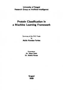
Category 9 Category 8 Category 9 Category 8 Fig. 3. Images randomly sampled from 10 categories and the corresponding segmentation results. Segmented regions are shown in their representative colors.

selected from 2−5 to 25 . For the regularization parameters c1 , c2 , c3 and c4 in binary class classification (9), we let c1 = c2 and c3 = c4 , with each of them being selected from 2−5 to 25 . For c1 and c2 in multi-class classification (36), we find them from 2−5 to 25 . As in [2], [12], [45], the averaged results of 10fold cross-validation with 5 independent runs are summarized.

TABLE I ACCURACY ON M USK 1 AND M USK 2 DATASETS .

APR [1] EM-DD [21] mi-SVM [12]

B. Performance for Binary Class Classification We evaluate the performance of SMILE for binary class classification based on several publicly available benchmarks: the Musk dataset 1 for drug activity prediction, the Corel dataset 2 for image retrieval, and the 20 Newsgroup dataset 3 for text categorization. 1) Musk Dataset: The Musk dataset consists of the data of molecules. A molecule is considered as a bag and each molecular shape is regarded as an instance. The Musk dataset contains two subsets: Musk1 and Musk2. The Musk1 dataset has 47 positive bags and 45 negative bags with about 5.17 instances per bag. The number of instances per bag varies from 2 to 40. The Musk2 dataset has 39 positive bags and 63 negative bags with around 64.69 instances per bag. The number of instances in each bag ranges from 1 to 1,044. A total of 72 molecules is shared between Musk1 and Musk2. Each instance is represented by a 166-dimensional feature vector. We first compare SMILE with the baselines - APR [1], EMDD [21], mi-SVM [12], MI-SVM [12] and DD-SVM [32]. Table I reports the average accuracies, standard deviations and p-values on the Musk1 and Musk2 datasets. The best accuracy is in bold. The p-values are computed by performing the paired t-test comparing all other classifiers to SMILE under the null hypothesis that there is no difference between the testing 1 Available

at http://www.cs.columbia.edu/Andrews/mil/datasets.html at http://kdd.ics.uci.edu 3 Available at http://people.csail.mit.edu/jrennie/20Newsgroups/ 2 Available

MI-SVM [12] DD-SVM [32] SMILE R SMILE

Musk1 p-value 92.4 ± 0.7 0.387 84.8 ± 2.2 0.024 87.4 ± 1.8 0.037 77.9 ± 2.4