06P-192
New Approach to Turbocharger Optimization Using 1-D Simulation Tools Oldˇrich VÍTEK, Jan MACEK, Miloš POLÁŠEK Czech Technical University in Prague Josef Božek Research Center c 2006 SAE International Copyright °
ABSTRACT The paper deals with the investigation of turbocharger optimization procedures using amended 1-D simulation tools. The proposed method uses scaled flow rate/effficiency maps for different sizes of a radial turbine together with a fictitious compressor map. The compressor pressure ratio/efficiency map depends on compressor circumference velocity only and predicts the both compressor specific power and achievable efficiency. At the first stage of optimization, it avoids the problems of reaching choking/surge limits. It enables the designer to find a suitable turbine type under realistic unsteady conditions (pressure pulses in exhaust manifold) concerning turbine flow area. Once the optimization of turbine/compressor impeller diameters is finished, the specific compressor map is selected. The proposed method provides the fast way to the best solution even for the case of a VGT turbine. Additional features have been developed for the representation of scaled turbine and compressor maps. They are based on application of versatile regression functions. No recalculation of normalized curves is needed. The method is presented for the model of a one-loop hot gas stand (steady performance compressor/turbine optimization) and for a modelled engine with different compressors. The potential of optimized turbocharger is evaluated at simulated typical operation points for a passenger car equipped with a 4-cylinder 2 dm3 engine.
nations of turbine and compressor maps provided by turbocharger manufacturers. The paper deals with one of the possible ways, using a 1-D model of turbine [6], amended by a compressor map extrapolation and combined with a 1-D engine simulation package [1]. The main problems are listed in the following section, the newly developed tools are described and finally some results of turbocharger optimization are commented on.
IDENTIFICATION OF MAIN PROBLEMS The problems of turbocharger matching/optimization concern: • the matching of turbine flow area to provide sufficient turbine power for required boost pressure taking into account realistic isentropic compressor efficiency; • the matching of turbine/compressor diameters or blading angles to use the optimum turbine efficiency; • the use of a reasonable domain in a compressor map (between surge and choking limits – Figure 1), ideally in the area of maximum efficiency; • consideration of the impact of low-pressure exhaust and air ducts (filters, mufflers, exhaust aftertreatment devices) on turbocharger performance due to the pressure losses caused by them.
INTRODUCTION The current development of downsized, turbocharged engines calls for mastering more effective approach in finding an optimal turbocharger or two-stage system of turbocharging. The widely used trial-and-error method using a collection of turbocharger maps is not an ideal one because of non-transparent results. It does not provide hints for turbocharger amendment. The presented procedure of finding optimal turbocharger for an engine is based on authors’ experience with turbomatching (e.g., 0-D code [4]). An application of the procedure is relatively fast and allows for finding suitable turbocharger without a need to calculate all feasible combi-
Figure 1: Typical parts of compressor map.
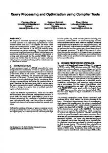
All optimization measures should take into account certain compromises, e.g., the pressure and temperature pulses in an exhaust manifold, operation domain with both different engine loads and speeds, and impacts of VGT concept on turbine efficiency at different rack positions. Nevertheless, the change of turbine flow area (e.g., by rack position or simply by turbine type change) causes a small variation of the turbine blade tip velocity ratio. This ratio is significantly influenced by compressor impeller diameter. Therefore, if a compressor impeller is not suitably fitted to a turbine, no change of turbine area will enable reaching the best turbine efficiency (Figure 8). The velocity ratio at fixed compressor specific power (enthalpy head) may be changed by variation of turbine/compressor diameter ratio (see below). Moreover, there are some feed-backs in the whole process of turbine/compressor matching. The most important one is a change of a fictitious effective flow area (or discharge coefficient) of a turbine due to change of blade tip velocity ratio x = u/cs during efficiency optimization – Figure 2.
• speeding-up iterative turbocharger optimizations starting with somewhat reasonable demands on compressor and turbine to find limits of engine performance, it could be applied to turbochargers not available at the time; • providing the demands or hints for a turbocharger manufacturer to design a turbocharger which is matched with a specific engine. The standard approach uses combinations of turbocharger maps available to the engine designer. The compromise found from them may be far from the optimum solution if no comparison to a theoretical optimum is done. In addition, the trial-and-error procedure is very slow and often constrained by limits of applied compressors and turbines. This may happen even in the time, when the final selection of compressor is not relevant. Therefore, at the initial stage, a particular compressor map is substituted by a map which represents a whole family of compressors. It does not take into account surge and choke limits to avoid the above mentioned problems. In the description above, ’theoretical’ means ’optimummatched’, using current typical state-of-the-art turbocharger design (i.e., achievable peak efficiencies of a turbine or a compressor). In the following sections, a way of finding such a ’theoretical’ optimum is outlined.
THEORETICAL BACKGROUND AND MAP REPRESENTATIONS COMPRESSOR Figure 2: Discharge coefficient of a radial turbine in dependence on blade tip velocity ratio and pressure ratio, a real set of operation points added (red curve), comparison to regression-represented map included in the graph (thin curves).
Applying angular momentum conservation, compressor enthalpy head (specific power) may be estimated using its impeller circumference velocity – Equation (1). 4hK = h0,K1 − h0,K2 = K1 u2K2 + K2 w2r uK2
Therefore, the matching of all parameters by systematic testbed experiments only is not effective. Even in the case of a VGT turbocharger, the change of turbine flow area (by changing a rack position) is not enough to determine optimum turbine/compressor diameter ratio. Moreover, the broad range of turbine area may cause compressor surging or efficiency decrease near to choking. Simulation may accelerate the whole process significantly if appropriate turbocharger maps are provided. Additional issues caused by these demands are: • reliable data from turbocharger manufacturers in sufficient ranges of all variables (especially concerning turbine u/cs and compressor map in the vicinity of low pressure ratios, even less than one); • a method of map representation in a simulation code; • methods of testing, calibration and validation of turbocharger performance at a real engine;
(1)
PK = 4hK m ˙K uK2 =
π D2K nT D 60
m ˙K π D2K b2K ρ2 µ ¶ πK TK1 pK1 ∼ 1+ ρ2 = rs TK1 TK2
w2r =
The first term on the right-hand side in Equation (1) is a dominant one, the second term is a correction for back-swept blades which are usually applied for more stable compressor performance. The coefficients must be evaluated from compressor map, usually by regression. The compressor speed dependence of these coefficients shows the reasonable assumptions of this representation (Figure 3). The overall errors of this substitution of real compressor map are usually less than 2%. The regression may be
Figure 3: Regression coefficients for compressor enthalpy head as a function of compressor speed.
Figure 5: Regression coefficients of compressor pressure curves at constant speed – compressor CZ 1364A.
applied if an extrapolation outside of the measured map is required. The important feature of the enthalpy head is the independence of pressure ratio.
all other speeds. This is usually an indication of possible errors. In this case, it seems that the measurement is not accurate enough at this compressor speed. On the other hand, another example is presented in Figures 6 and 7. In this case, there is no such a problem. What might be of interest is the fact that constant speed lines for higher compressor speeds are not monotonically decreasing. This is not a measurement problem, it is a typical feature of this compressor family.
Compressor isentropic efficiency may be found during simulation if pressure ratio is expressed as a function of compressor speed. Polynomial fraction functions (Equation (2)) are suitable for it as authors’ experience has showed. πK =
a nred m ˙ red + b 2 −c nred m ˙ red + d nred m ˙ red + 1
(2)
Linear regression procedures may be used for this aim after the transformation: the denominator in Equation (2) is used for multiplying pressure ratio. The accuracy of this representation is relatively high (it is an extrapolation) – Figure 4 and Figure 6.
Figure 6: Representation of compressor pressure curves at constant speed by regression compared to measured data and extrapolated to full choking – compressor CZ 6268ACS.
Figure 4: Representation of compressor pressure curves at constant speed by regression compared to measured data and extrapolated to full choking – compressor CZ 1364A.
The compressor efficiency is computed according to Equation (3). ηKs =
The extrapolation to sub-unity pressure ratios is possible and the errors in measurement of compressor map are clearly shown during it (Figure 4). The speed lines must not intersect. In the presented example, the data at the speed of 100 000 min−1 seem to be slightly distorted. It is demonstrated by the regression coefficients a, ..., d as well – Figure 5. Especially coefficient c is quite different at speed 100 000 min−1 when compared with its value for
cpK
h0,K1 − h0,K2 µ κK −1 ¶ κK T0,K1 πK −1
(3)
For the aims of ’theoretical’ compressor simulation in the stage of the primary turbine matching, a fictitious compressor with state-of-the-art peak efficiency, but without any surge or choke limits, may be created from these relations. Only after a turbine has been set, the real compressor is implemented into simulation.
Figure 8: Isentropic efficiency of a radial turbine in dependence on blade tip velocity ratio and pressure ratio, a real set of operation points added (red curve), comparison to regression-represented map included in the graph (thin curves).
Figure 7: Regression coefficients of compressor pressure curves at constant speed – compressor CZ 6268ACS.
TURBINE TURBOCHARGER OPTIMIZATION
The radial turbine simulation is more difficult due to the mentioned dependence of flow features (e.g., discharge coefficient applied to a fictitious nozzle of constant flow area, Figure 2) on a velocity ratio, which is a subject of efficiency optimization (see next subsection). The fictitious isentropic velocity, which is used in a velocity ratio definition, is defined in Equation (4). c2s h0,T 1 − h0,T 2 = h0,T 1 − h0,T 2s = 2 ηT s s µ ¶ cs =
(4)
1−κT κK
2 cpT T0,T 1 1 − πT
Besides, there is a need to represent turbine maps (both flow and efficiency) as accurately as possible during the simulations. The method of predictive extrapolation of both values from experiments was already described in detail in [6]. The results can be represented by regressions, not using any normalized maps. The useful form of regressions is (for both isentropic efficiency and discharge coefficient) written in Equation (5).
ηT s =
N X
ai πTei xfi = a0 + a1 πT + a2 πT2 + a3 πT3
(5)
i=1
+a4 x + a5 x2 + a6 x3 + a7 x4 + a8 πT x + a8 πT2 x The measured and regression-represented curves are shown in Figure 2 and Figure 8. Although this representation provides a sufficiently accurate tool for simulation input, it is not usable for extrapolations unless they are calculated in advance by the fully 1-D turbine model. Therefore, the next step in simulation tool development should be the implementation of this model in it. This case will be published in the future.
The above mentioned feed-back between turbine efficiency and discharge coefficient will be explained in this section. The power balance of a free-shaft turbocharger yields Equation (6). ηmT D m ˙ T (h0,T 1 − h0,T 2 ) + m ˙ K (h0,K1 − h0,K2 ) = 0 (6) Using it together with isentropic speed definition and compressor isentropic efficiency definition, the result yields Equation (7). µ κK −1 ¶ c2 m ˙T κ cpK T0,K1 πK K − 1 = ηKs ηT s ηmT D s (7) 2 m ˙K The ratio of flow rates is constant and close to unity (except for waste-gating). It means that the isentropic speed is determined for required boost pressure and at reasonable state-of-the-art efficiencies. Since it is closely bound to the turbine flow rate (see relation to turbine-inlet pressure and temperature in Equation (4)), the turbine flow area is determined, as well. On the other hand, it is possible to derive Equation (8) from angular momentum equation. K1 u2K2 + K2 w2r uK2 = ηT s ηmT D
c2s m ˙T 2 m ˙K
(8)
Since the second term on the left-hand side of the Equation (8) is not important, ratio of uK2 /cs is given by this equation. The obvious relation among speed, impeller diameters and circumference velocities yields required diameter of a turbine, if optimum velocity ratio and compressor dimensions are known. These associations should be kept in mind during turbocharger matching by means of simulation. Before the specific procedures for 1-D engine simulation codes are described, an often-neglected phenomenon should be mentioned. The aim of any turbocharger optimization is to find a combination of turbine and compressor, providing demanded
boost pressure at known engine exhaust gas flow-rate and temperature. An optimized turbocharger requires the lowest exhaust manifold backpressure for this aim. Ideally, some of the heat rejected from a thermodynamic cycle is regenerated back to the cycle work. All the mentioned relations deal with pressure ratios only, nevertheless. The sources of any pressure losses outside of a turbocharger may be very important for the result of optimization, i.e., the difference between boost and exhaust pressure.
data and instantaneous pressure ratio at a turbine using isentropic pressure-temperature dependence. Simulations in a 1-D code have proven that this simplification may be used for typical car and truck engines with no scavenging. The values of flow rate and power are integrated and compared to measured or simulated ones. The procedure is very useful in testing map reliability and its interpretation in a simulation code. An example of results for a moderately turbocharged truck engine is in Figure 10.
An example of a quite realistic case is presented in Figure 9. State-of-the-art HD diesel turbocharger (overall efficiency 50%) is concerned. Exhaust gas temperature is 900 K and nominal pressure losses in compressor air inlet are 10 kPa at nominal power. Pressure losses dependence on flow rate is supposed to be quadratic for air inlet flow. Exhaust aftertreatment losses and muffler ones are 30 kPa at nominal power. Mainly linear dependence on flow rate is expected for the exhaust devices (laminar flow in a DPF).
Figure 10: Traces of pressure ratio, velocity ratio, isentropic efficiency, discharge coefficient and turbine power evaluated from a measurement.
The authors’ institution is able to measure an instantaneous turbine speed. It will be employed to these evaluations as well, giving another independent source of validation data. Figure 9: Pressure ratios and absolute pressure at a turbocharger – impact of pressure losses on available boost pressure.
The fatal impact of apparently reasonable pressure losses is quite clear (Figure 9). Although the turbocharger itself is able to give a positive pressure difference between inlet and exhaust ducts, the pressure losses even limit the achievable boost pressure.
MATHEMATICAL MODEL The presented results were obtained by means of numerical simulation. Both a one-loop hot gas stand model (to test turbocharger in a close loop) and an engine model were created in 0-D/1-D code GT-Power [1].
ONE-LOOP HOT GAS STAND MODEL
TURBINE PARAMETERS ASSESSMENT Considering all uncertainties in turbocharger map implementation, a calibration method development seems to be advisable. For this reason, an inversed algorithm has been programmed using regression representation of manufacturer-delivered or predicted turbine map based on Equation (5). Static pressure downstream of turbine, instantaneous speed, the isentropic enthalpy head, velocity ratio, efficiency, discharge coefficient, turbine flow rate and power are calculated from turbine inlet total pressure and turbine inlet temperature. In the case of measured values, temperature is calculated from the measured averaged
A model of the one-loop hot gas stand (SAE J922 and SAE J1826 for more detailed information about terminology) was created in GT-Power (Figure 11) to test whether a compressor fits well with a given turbine. A turbocharger is tested in a similar way as it is required in the SAE J1826. An amount of fuel injected in a burner is controlled for achieving desired mass flow or turbine pressure ratio. Normalized blade speed ratio is computed applying Equation (10). Blade speed ratio is calculated using Equation (9). Moreover, a parameter called ’specific speed’ is computed according to Equation (11). This parameter may be used for evaluation of the turbine or compressor design. The lower the value of specific speed is, the ’more’ radial
design of rotor blades should be applied. x=
uT 1 cs
(9)
xnorm =
x xopt
(10)
¡ ¢1 nT D V˙ 2 nq = 333.3 60 ³ c2s ´ 43
(11)
Bore Stroke Compression Ratio Charging Fuel Injection Configuration No. of Intake Valves No. of Exhaust Valves
[mm] [mm] [1]
81 95.5 16 Turbocharged Diesel Direct, Common-rail R4 2 1
2
Table 1: Main engine parameters for the 2.0L turbocharged DI engine.
achieve best possible engine efficiency under given limiting conditions. The parameters to be optimized ware injection timing and VGT rack position. Minimum air excess, maximum in-cylinder pressure, maximum turbocharger speed and turbine inlet temperature ware constraining factors. In general, compressor surge is a limiting factor as well. In this case, it was never a problem (see more detailed comments in the following section). Maximum Torque Engine Speed of Max. Torque Maximum Power Engine Speed of Max. Power
[N.m] [1/min] [kW] [1/min]
270 2000 - 3000 87 3500 - 4000
Table 2: Required output parameters of 2.0L engine.
Figure 11: GT-Power one-loop hot gas stand model.
ENGINE MODEL The main engine parameters are summarized in Table 1. It is a 2.0 liter passenger car turbocharged diesel DI engine (Figure 12). Its geometrical data (e.g., manifold layouts, valve lifts and flow properties) are based on real engine data. The engine itself is still being developed. The engine is equipped with a variable geometry turbine (VGT), intercooler, and both low pressure and high pressure EGR circuit including EGR intercooler. All remaining parameters were estimated using the authors’ experience with similar engine models. To obtain qualitatively correct results, predictive models have to be applied. For combustion parameters, the Woschni recalculation was used to take into account engine speed and air excess. For in-cylinder heat transfer, the Woschni formula [8] is applied and a simple finite element method (FEM) solver is used to calculate heat transfer through the walls. Mechanical losses are computed according to semi-empirical formula [2]. The required engine output parameters under full load are plotted in Table 2. The engine setting was optimized to
Figure 12: GT-Power engine model.
Finally, optimized engine setting was found for highway driving. Required engine part load parameters are summarized in Table 3 (gearbox ratios were estimated). Once again, both injection timing and VGT rack position were
optimized for lowest BSFC. BMEP at 90 km/h at 4th gear Engine Speed at 90 km/h at 4th gear BMEP at 130 km/h at 5th gear Engine Speed at 130 km/h at 5th gear
[bar] [1/min] [bar] [1/min]
4.46 2104 9.22 2167
Table 3: Required engine parameters for highway driving (gear ratios estimated).
PROCEDURE MATCHING
FOR
a GT-Power parameter which is used to distinguish different turbine stator geometry. In general, the higher the rack position value, the higher turbine swallowing capacity. This means that an optimal compressor is being found for one particular VGT setting when one-loop hot gas stand testing is performed. It should be mentioned that the VGT setting is likely to vary under more realistic engine operating conditions.
TURBOCHARGER
In this section, the procedure for turbocharger matching is described. Firstly, selected compressor maps were checked on the one-loop hot gas stand if they were suitable to be applied with a given turbine. The compressor maps were created as described above. Secondly, turbochargers were added to an engine model and full load curve was optimized for the lowest engine fuel consumption. Constants K1 and K2 are the most important compressor parameters which describe a compressor with respect to enthalpy head (Equation (1)). See Figure 13 for dependency of K1 and K2 on compressor speed which was derived from real compressor map by means of regression.
Figure 13: Dependence of constants K1 and K2 (applied in Equation (1)) on compressor speed.
Parameter b2K is used to tune the compressor regression model so that compressor constant speed line angle (deviation from horizontal line) is the same as for a real compressor map. This is quite an important fact. See Figures 14 and 15 for real compressor characteristics and Figures 16 and 17 for numerical model compressor characteristics. The black line in these figures represents operating points at which turbochargers are numerically tested on the one-loop hot gas stand. The turbine is the same for all data concerning one-loop hot gas stand testing. The applied VGT turbine rack position is the highest efficiency one from all rack positions. When performing engine tests, the rack position is allowed to change. The rack position is
Figure 14: Real compressor speed characteristics (black line represents compressor operating points for one-loop hot gas stand model computation).
Figure 15: Real compressor efficiency characteristics (black line represents compressor operating points for one-loop hot gas stand model computation).
It is also necessary to make sure that compressor operating points lay under a surge line and in a region of constant speed curves being nearly lines. Therefore, the compressor characteristics look like as in Figures 16 and 17. Such characteristics may look ’unrealistic’ but they represent the whole family of compressors from which a user should choose in the end. Compressor efficiency contours are almost independent of compressor mass flow. It should be stressed again that the compressor maps based on the above described mathematical model are valid in the region where compressor constant speed curves are lines only (left part of the map in Figures 16 and 17). The right
region of these maps, where compressor constant speed curves are ’turned down’, is extrapolated by the applied code (GT-Power). Compressor operating points should not lay in the right region. The compressor efficiency is another tuning factor. It should correspond to the real compressor value. In the presented examples (Figures 16 and 17), it is a bit lower when compared to the real compressor maximum efficiency. The efficiency is constant in the expected operational region to see the highest possible potential at each engine speed under any engine load. The constant value of compressor efficiency is the same for all compressor variants.
Figure 16: Numerical model compressor speed characteristics (black line represents compressor operating points for one-loop hot gas stand model computation) for reference diameter of 51 mm.
Figure 17: Numerical model compressor efficiency characteristics (black line represents compressor operating points for one-loop hot gas stand model computation) for reference diameter of 51 mm.
Finally, when a set of compressor characteristics is created, another set can be easily derived by means of changing compressor reference diameter which means changing uK2 (Equation (1)). To summarize all created compressor characteristic sets, the reference diameters of 49, 51, 53, 57 and 60 mm were applied. For each of them, a calculation of the one-loop hot gas stand test and engine optimization were performed. The last step of the method is to identify the best compromise solution and then to find a set of real compressor maps (from all available maps of different manufactures) which are similar to simplified maps. After that, calculation of desired data (full load, part load, etc.) has to be performed to obtain the final results. In general, similar approach can be taken for finding suitable turbine (even VGT type). The methodology was published in [6]. In general, when selecting a real compressor, its useful operating range is limited by both the surge line and the choke limit. These were not taken into account when creating simplified maps representing the whole compressor family. The compressor family consists of compressors which may differ in design but they have the same reference diameter of rotor. As a result of that, when computing data for the whole engine speed range and when the real compressor map is used, some operating points may lay beyond surge limit or may be placed too close to both surge or choke limit. This may limit application of potentially optimal combination of compressor and turbine. It may even lead to selection of a different turbocharger. If considering presented engine example (Table 1), this was never the case, although several real compressor maps were tested. This statement was valid even if a higher load was desired when compared with Table 2. Averaged compressor operating points for a real compressor map at engine full load are plotted in Figure 18. It is clear that the simplified compressor map is not capable of representing real compressor under any operating conditions. Instead, it corresponds to the best possible design from the whole compressor family for a given compressor reference diameter. Its application requires some user experience. The optimal turbocharger, which is a combination of compressor and turbine, might be found by means of the presented procedure. However, if real turbocharger is applied, the results will be slightly worse, especially for compressor
Figure 18: Real compressor averaged operating points plotted in compressor efficiency map (engine is fully loaded, Table 2) – example of application of possible real compressor map.
Figure 19: Dependency of turbine normalized blade speed ration xnorm on turbine speed at one-loop hot gas stand for all compressor variants.
operating points which lay in the regions of lower efficiency (near surge line or near choke limit).
DISCUSSION OF RESULTS In this section, all the results are presented. First, the oneloop hot gas stand computed data for each compressor variant are commented on. Second, the results of engine testing for the full load curve and highway driving are discussed.
ONE-LOOP HOT GAS STAND MODEL The most important result of this subsection is a comparison of turbine normalized blade speed ratio (NBSR defined in Equation (10)) as a function of turbine speed, which is plotted in Figure 19. It is clear that compressors with various reference diameters load the turbine differently. This leads to significantly different NBSRs. From this point of view, the optimum compressor reference diameter is 49 mm. This statement is based on the empirical fact that optimum compressor (for given turbine) loads the turbine on the one-loop hot gas stand in such a way that NBSR approximately equals to 1. This is confirmed in Figure 21 – turbine operates in region of better efficiency for small compressors. The efficiency of the compressor itself is almost identical when different compressor variants are compared (Figure 20). As mentioned above, it is constant in the expected operational region. Specific compressor and turbine speeds are plotted in Figure 22 and 23 respectively. Empirical knowledge shows that turbine specific speed should be approximately between 40 and 50 for current turbine designs. This also confirms that compressors with the reference diameter of 49 and 51 mm seem to be the ideal choice for the given turbine.
Figure 20: Dependency of compressor efficiency on compressor speed at one-loop hot gas stand for all compressor variants.
Figure 21: Dependency of turbine efficiency on turbine speed at one-loop hot gas stand for all compressor variants.
ENGINE MODEL
Figure 22: Dependency of compressor specific speed on compressor speed at one-loop hot gas stand for all compressor variants.
The integral results concerning engine testing are presented in Figures 24-30. It should be stressed that the optimum engine setting was applied. Both injection timing and VGT turbine rack position were optimized for the highest engine efficiency. It is possible to fulfill the BMEP requirement (Table 2) for all compressor variants. Engine specific fuel consumption (BSFC) is presented in Figure 24. As the engine is concerned, the best compressor variants are those with the reference diameter of 49, 51 or 53 mm. It has to be stated that the overall engine efficiency is influenced by many factors (and applied turbocharger is only one of them). On the other hand, the only difference among the presented variants is the compressor itself. The reasons for different engine efficiencies can be found in Figures 25-30. Generally speaking, the optimum engine setting is a compromise of many different, and usually contradictory parameters which are commented on in the following paragraphs. There are differences in the pumping work necessary for engine in-cylinder gas exchange (Figure 25) which are influenced mainly by mass and energy transfer between the engine and the turbocharger. The optimum engine air excess is plotted in Figure 26. The higher the air excess, the faster combustion and hence better indicated efficiency of high-pressure phase of an engine cycle. For variants with the reference diameter of 53, 57 and 60 mm, the optimum air excess at lower engine speed is significantly higher when compared with other variants. On one hand, it improves combustion speed. On the other hand, negative pumping work is large. Mechanical losses differ slightly as well. The main reason is the difference in maximum in-cylinder pressure (Figure 28) which is used in the ChenFlynn model. In-cylinder heat transfer (Figure 27) is another important factor. The differences are not negligible and they are caused by different in-cylinder temperature patterns during a high-pressure phase of the engine cycle. Finally, the cycle averaged efficiencies of both compressor (Figure 29) and turbine (Figure 30) are important in terms of the pumping work and intercooler heat losses.
Figure 23: Dependency of turbine specific speed on turbine speed at one-loop hot gas stand for all compressor variants.
Figure 24: Dependency of engine BSFC on engine speed for all compressor variants (optimized engine setting is applied).
Figure 25: Dependency of engine pumping MEP on engine speed for all compressor variants (optimized engine setting is applied).
Figure 26: Dependency of engine air excess on engine speed for all compressor variants (optimized engine setting is applied).
Figure 27: Dependency of in-cylinder heat transfer (averaged for one engine cycle) for all cylinders on engine speed for all compressor variants (optimized engine setting is applied).
Figure 28: Dependency of maximum in-cylinder pressure on engine speed for all compressor variants (optimized engine setting is applied).
Figure 29: Dependency of averaged compressor efficiency on engine speed for all compressor variants (optimized engine setting is applied).
Figure 30: Dependency of averaged turbine efficiency on engine speed for all compressor variants (optimized engine setting is applied).
Figure 31: Dependency of VGT turbine rack position on engine speed for all compressor variants (optimized engine setting is applied).
From the turbocharger point of view, it is important that the turbine operates at the best possible region. In other words, that turbine efficiency operating curve should lay near the optimum value of NBSR which of course equals to 1 according to Equation (10). The turbine operating points should mainly be located in the region of NBSR greater than 1 to keep high turbine efficiency at high enthalpy heads (as it is the case in Figure 33 for the reference compressor diameter of 49 mm). From the qualitative point of view, the turbine operating curve is shifted more to the left in the turbine operating diagram (Figures 32 and 33) if the compressor reference diameter is larger. A maximum enthalpy head corresponds to the lowest NBSR. Therefore, this point should lay as close as possible to a point of maximum turbine efficiency. That is why the averaged turbine efficiency is better for all computed points (with an exception of 4000 rpm) for smaller compressor reference diameters (Figure 30).
Figure 32: Dependency of instantaneous turbine efficiency on instantaneous turbine normalized blade speed ratio (NBSR) for all compressor variants (optimized engine setting is applied) at engine speed 2000 rpm.
The proposed method is able to set an arbitrary correlation between compressor reference diameter and its efficiency. If no particular data are available for calibrating it comparing different compressors of the similar design, it is recommended to set the compressor efficiency independent
Figure 33: Dependency of instantaneous turbine efficiency on instantaneous turbine normalized blade speed ratio (NBSR) for all compressor variants (optimized engine setting is applied) at engine speed 3000 rpm.
of compressor reference diameter. This approach was applied in this case. Moreover, compressor efficiency is constant in the expected operational region. This enables to see the influence of turbine operating curve (Figures 32 and 33). With respect to the highway driving optimizations, they are presented in Figures 34-38. See Table 3 for required engine speed and BMEP. Once again, the optimum engine setting is the overall result of different phenomena. As it is the case under engine full load, the variants with the compressor reference diameter of 49 and 51 mm seem to be optimal from the overall engine efficiency point of view (Figure 34). The main reasons for this statement can be found in Figures 35-38. There are significant differences in pumping work (Figure 35) which are mainly caused by different optimum air excess for each variant (Figure 36, this sets requirements for air mass flow rates) and different compressor and turbine efficiencies (Figures 37 and 38 respectively). Especially the variation of turbine averaged efficiency in the Figure 38 is quite significant. When optimizing engine setting for the vehicle speed of 90 kmph, engine load is so low that compressor operating points are not located in the region of constant compressor efficiency any more. Hence, compressor efficiency is another important factor which contributes to better engine efficiency for smaller reference diameter variants. When performing optimization for vehicle speed of 130 kmph, compressor efficiency is almost constant. The results are qualitatively the same as for lower engine speed, the differences in BSFC are smaller. Turbine operating curves for all compressor variants are plotted in Figures 39 and 40. The influence of both friction and heat transfer is not very important. To sum up, a compromise has to be made in selecting an optimum compressor. In this particular case, an optimum compressor reference diameter seems to be 51 mm. Such a compressor performed well in the one-loop hot gas stand test. When applied to the whole engine model, the overall engine efficiency was the highest one at each engine speed.
Figure 34: Dependency of BSFC on vehicle speed for all compressor variants (optimized for highway driving – see Table 3).
Figure 37: Dependency of averaged compressor efficiency on vehicle speed for all compressor variants (optimized for highway driving – see Table 3).
Figure 35: Dependency of engine pumping MEP on vehicle speed for all compressor variants (optimized for highway driving – see Table 3).
Figure 38: Dependency of averaged turbine efficiency on vehicle speed for all compressor variants (optimized for highway driving – see Table 3).
Figure 36: Dependency of engine air excess on vehicle speed for all compressor variants (optimized for highway driving – see Table 3).
Figure 39: Dependency of instantaneous turbine efficiency on instantaneous turbine normalized blade speed ratio (NBSR) for all compressor variants (optimized engine setting is applied) at vehicle speed of 90 kmph at 4th gear.
and during engine matching. The example of application of the above described method has been presented. First, the one-loop hot gas stand tests have been performed to check whether compressor characteristics ware suitable to be applied together with given turbine. Second, engine optimizations under full load and part load have been performed to see overall effect on engine output parameters. In the presented case, the existing variable geometry turbine (VGT) has been employed.
Figure 40: Dependency of instantaneous turbine efficiency on instantaneous turbine normalized blade speed ratio (NBSR) for all compressor variants (optimized engine setting is applied) at vehicle speed of 130 kmph at 5th gear.
CONCLUSION A method for turbocharger optimization using a fictitious compressor map for preliminary optimization steps has been developed and tested. Its main meaning is in understanding the links between compressor and turbine performance and finding options for the best state-of-the-art turbocharger even if its map does not exist. Moreover, the method is faster than mechanical combining of available maps, using a trial-and-error approach. As a side effect of this, the big impact of today’s usual pressure losses on a turbocharger performance was confirmed. It may result in a limitation of boost pressure even if turbine inlet pressure is further increased. The method of regression-based representation of compressor and turbine maps has been developed and tested as well. It is based on authors’ experience with turbocharger matching using 0-D approach which was successfully tested in the past using 0-D code [4]. The presented method is generalized to be suitable for 0-D/1-D codes. It is useful not only for simulation codes and reliable compressor map extrapolations but also for the experiment evaluation and testing of the map representation in 1-D codes. Correlation between compressor reference diameter and its efficiency has not been generally verified yet. The authors are aware of the fact that this phenomenon might influence the results. In this case, constant compressor efficiency was prescribed in the expected operational region. It was the same for each compressor variant. The main reason for that was the requirement to see the highest potential at each engine speed under any engine load. In the future, the complete turbine map prediction should be included in 1-D codes. If validated by experiments at a turbine, it will be able to couple 1-D gas dynamics phenomena with those of a quasi-steady turbine performance. It will provide deeper insight into the turbocharger operation. This may be useful for its optimization at a manufacturer
As one can expect, the final decision of selecting a suitable compressor is a compromise of many factors depending on user requirements. As it is clear from the presented results, compressor reference diameter of 51 mm is the best compromise. It performed well both on the one-loop hot gas stand and in the engine. However, if higher engine BMEP is required (at the time, it is usual to have engine producing over 22 bars of BMEP, which is approximately torque of 340 Nm for the 2.0L engine), the smaller compressors cannot provide enough mass flow and therefore the larger ones have to be used. In general, the analogical approach can be applied for finding optimum turbine (even VGT type). It is also based on suitable regression functions which can represent basic turbine properties. More details can be found in [6]. Therefore, the optimum turbocharger (both compressor and turbine) for specific engine needs can be derived. The final step of the method is to find real maps for both compressor and turbine which are as closely matched to the theoretical ones as possible. After selecting real turbocharger data, recalculation should be performed to obtain final results.
ACKNOWLEDGEMENT This work has been supported by the Josef Božek Research Center, No. 1M68400770002. This help has been gratefully appreciated.
REFERENCES [1] GT-Power Users’s Manual, GT-Suite version 6.0. Gamma Technologies Inc., March 2003. [2] Chen, S. and Flynn, P. Development of a Single Cylinder Compression Ignition Research Engine. SAE Technical Paper Series. Paper 650733. [3] Heywood, J. B. Internal Combustion Engine Fundamentals. McGraw-Hill series in mechanical engineering, printed in USA. McGraw-Hill, 1988. ISBN 0-07028637-X. [4] Macek, J. Program for Thermodynamic Cycle Simulation of Turbocharged Engine – OBEH, version 00-I, 2000. Program library – Ú 220. [5] Macek, J. and Kliment, V. Gas Turbines, Turbochargers and Fans. CTU in Prague, 1992 - 1996. ISBN 80-0100840-1. (In Czech).
[6] Macek, J., Vávra, J., and Vítek, O. 1-D Model of Radial Turbocharger Turbine Calibrated by Experiments. SAE Technical Paper Series, March 2002. Paper 2002-010377. [7] Vítek, O. and Polášek, M. Tuned Manifold Systems – Application of 1-D Pipe Model. SAE Technical Paper Series, March 2002. Paper 2002-01-0004. [8] Woschni, G. A Universally Applicable Equation for the Instantaneous Heat Transfer Coefficient in the Internal Combustion Engine. SAE Transactions, Vol. 76:3065, 1967.
CONTACT Oldˇrich VÍTEK
INDICES AND ACRONYMS BMEP
... brake mean effective pressure
BSFC
... brake specific fuel consumption
BSR
... blade speed ratio
CH
... cooling
DI
... direct injection
DPF
... diesel particulate filter
EGR
... exhaust gas recirculation
FEM
... finite element method
HD
... heavy duty
K
... compression; compressor
M
... engine
MEP
... mean effective pressure
NBSR
... normalized blade speed ratio
norm
... normalized
Czech Technical University in Prague Josef Božek Research Center Technická 4 CZ - 166 07 Prague Czech Republic
opt
... optimum
red
... reduced to the reference pressure and temperature
ref
... at zero enthalpy
phone: +420 224 352 507 e-mail:
[email protected]
s
... isentropic
T
... turbine; termodynamic
VGT
... variable geometry turbine
1
... upstream/inlet
2
... downstream/outlet
SYMBOLS A
... flow area
[m2 ]
c
... speed
[m.s−1 ]
h
... specific enthalpy
[J.kg −1 ]
m
... mass
[kg]
nM
... engine speed
[min−1 ]
nT D
... turbocharger speed
[min−1 ]
p
... pressure
[P a]
P
... power
[W ]
r
... specific gas constant
[J.kg −1 .K −1 ]
T
... temperature
[K]
u V˙
... circumferential speed
[m.s−1 ]
... volume flow
[m3 .s−1 ]
x
... blade speed ratio
[1]
α
... crank angle
[degCA]
ε
... compression ratio
[1]
η
... efficiency
[1]
κ
... isentropic exponent
[1]
π
... pressure ratio (sometimes substituted by symbol ’pi ’ in figure legends) ... density
[1]
ρ
[kg.m−3 ]