dynamics and the tracking error. The control law then depends on these estimates. Therefore, this results in a new version of the sliding mode control of robot ...
IEEE TRANSACTIONS ON ROBOTICS AND AUTOMATION, VOL. 9, NO. 2, APRIL 1993
208
Short Papers A Sliding Mode Controller with Bound Estimation for Robot Manipulators Chun-Yi Su and Tin-Pui Leung Abstract-A sliding mode control algorithm combined with an adaptive scheme, which is used to estimate the unknown parameter bounds, is developed for the trajectory control of robot manipulators. Simulation results show the validity of accurate tracking capability and robust performance.
I. INTRODUCTION In recent years increasing attention has been given to controller designs of robot manipulators that utilize the theory of variable structure system (VSS) [I]-[ 121. VSS (see [ 131 for a recent review) is based on the concept of an attractive manifold of the underlying state or error vector space on which the desired dynamic behavior is assured. These systems are a special class of nonlinear systems characterized by a discontinuous control action which changes structure upon reaching a sliding surface s ( s ) = 0. A fundamental property of VSS is the sliding motion of the state on the "attractive" manifold. During this sliding motion the system has invariance properties, yielding motion which is independent of certain system parameter variations and disturbances. Among developed control algorithms using the theory of VSS, several approaches have been considered. Some use the method of the hierarchy [I]-[3], others do use the Lyapunov stability method [4]-[9], and the linearizable method [IO], [ I I]. But all the derived control laws are based on the restrictive assumption that the bounds of the variations of the plant parameters are known a priori. In many practical situation. even if the bounds can be learned, they may be conservative. The implementation of the control law, based on these conservative bounds, may results in impractically large control magnitudes. Furthermore, these excessive controls will lead to large control chattering which may excite high-frequency unmodelled dynamics in the system. In this paper, a sliding mode controller with the bound estimation is proposed for accomplishing trajectory control of robot manipulators. The proposed method is based on the linear parameterization approach [ 141, [ 151, which decomposes the manipulator dynamic equations into the product of two quantities: a constant unknown vector of manipulator parameters, and a known nonlinear function of the manipulator dynamics, called the regressor matrix. By using the regressor, a new sliding mode control law is designed. We assume here that the system matrix is completely unknown and no information on its possible size is given. The bounds of the unknown parameters, which are needed for calculating the switching gain, are not required known here. Instead, an adaptive algorithm is constructed such that the bounds are generated as a function of the state of the Manuscript received January 2, 1991; revised February 25, 1992. C. Y. Su is with the Department of Automation, South China University of Technology, Guangzhou 510641, People's Republic of China, and is on leave at the Department of Mechanical Engineering, University of Victoria, Victoria, BC, V8W 3P6, Canada. T. P. Leung is with the Department of Mechanical and Marine Engineering, Hong Kong Polytechnic, Hung Hom, Kowloon, Hong Kong. IEEE Log Number 9207359.
dynamics and the tracking error. The control law then depends on these estimates. Therefore, this results in a new version of the sliding mode control of robot manipulators. Usually, some unmodelled external forces, frictions, etc., may effect the stability. Thus, the controller should be robust in the presence of such uncertainties. Customarily, the uncertainties in the VSS trajectory tracking designs are assumed to be bounded by a constant. This assumption may be restrictive as far as friction forces are concerned. Uncertainties are, in general, functions of the system states. In this paper, the robustness with respect to the uncertainties is analyzed, where the uncertainties are assumed to be unbounded and fast-varying. Analysis results show that the robustness is guaranteed. The organization of this article is as follows. In Section I1 the robot dynamics and its structure properties are reviewed. Section 111 presents a sliding mode control algorithm with bound estimation, and the robust analysis with respect to uncertainties is given. The elimination of chattering is also discussed in this section. Section IV gives the extension to Cartesian space. Finally the simulation results are given in Section V. 11. MANIPULATOR DYNAMIC PROPERTIES A manipulator is defined as an open kinematic chain of rigid links. Each degree of freedom of the manipulator is powered by independent torques. Using the Lagrangian formulation, the equations of motion of an n-degree-of-freedom manipulator can be written as
+
(1)
where q E R" is the generalized coordinates (joint positions); D ( q ) E R'lX7' is the symmetric, bounded, positive definite inertia matrix; vector B ( q , q ) q E R" presents the centripetal and Coriolis torques; G ( q ) E R" is the vector of gravitational torques, which is bounded C' function; and U E R" is the vector of applied joint torques. The robot model (1) is characterized by the following structural properties, which are of importance to our stability analysis. Property 1: There exists a vector a E RnZ with components depending on manipulator parameters (masses, moments of inertia, etc.), such that
+ B ( q . q ) v+ G ( q )= @ ( q . q . v . w ) a
D(q)u
(2)
where E R n X mis called the regressor [14], [15],v E R" is a vector of smooth functions. This property means that the dynamic equation can be linearized with respect to a specially selected set of manipulator parameters, thus constituting the basis of the linear parameterization approach [141, ~ 5 1 Property 2: Using a proper definition of matrix B ( q . q ) , both D ( q ) and B ( q , j . )in (1) satisfy
z T ( D- 2 B ) z = 0. V z E R"
(3)
with z r the transposition of z. That is, ( h - 2 B ) is a skew-symmetric matrix [15], [16]. In particular, the elements of B ( q , q ) may be defined as [15], [I91
1042-296X/93$03.00 0 1993 IEEE
I
+
D(q);i B ( q . q ) q G(q)=
IEEE TRANSACTIONS ON ROBOTICS AND AUTOMATION, VOL. 9, NO. 2, APRIL 1993
Property 2 is simply a statement that the so-calledfictitiousforces, defined by B ( q , q ) q ,do not work on the system [19]. Remark: The structure properties of the robot dynamics presented above have been used to design a sliding mode controller for the trajectory tracking problem. By using Property 2, a simple sliding mode controller was presented [4]. Other classes of the sliding mode controllers [7]-[9] were proposed with the help of Properties 1 and 2.
209
Remark: The role of the linearity-in-parameter expressed by (7) is twofold. Firstly, it makes the design possible for isolating the unknown parameters from the robotic dynamics. Secondly, by using the regressor matrix the explicit sliding mode control form can be easily expressed, which is, in general, difficult [1]-[3]. With the construction of U in (8), we obtain the following sliding mode equation
D s = @$ - @ a - Bs - I i d s
111. SLIDING MODE CONTROLLER WITH BOUNDS ESTIMATION A. Controller Design
The considered tracking problem is stated as follows: Knowing desired trajectory qd E R", qd E R", and qd E R", with some or all the manipulator parameters unknown, determine a control law U and a sliding surface s = 0 such that sliding mode occurs on the sliding surface, the tracking error q = q - qd E R" has a prescribed transient response and it goes to zero asymptotically as t -+ 03. In this paper the sliding surface s = 0 is chosen as hyperplane, where s=q
+ Aq
(4)
where A is a positive definite matrix whose eigenvalues are strictly in the right-hand complex plane, and q ( t ) = q ( t ) - q d ( t )is the tracking error vector. If the sliding mode exists on s = 0, then from the theory of VSS, the sliding mode is governed by the following linear differential equation whose behavior is dictated by the sliding hyperplane design matrix .I:
(1 1)
which is obtained by subtracting (7) from both side of (l), and using the fact that s = 4 - q,. Now we are ready to state our main results. Theorem 1: Consider robotic system (1) with sliding surface (4) and control laws (8), (9), and (IO), then the tracking error q ( t ) converges to the sliding surface and is restricted to the surface for all subsequent time. Pro08 Consider the following Lyapunov function
where 17% is constant satisfying q Z 1 lazlrtherein at is the ith components of the vector (Y defined in (7). +jzis its estimation. Differentiating (12) with respect to time along the solution of (11) gives
V = s T ( @ $- @a- I i d s - B s )
;
+ -sT (:t-D
)
s
m
1=1
Obviously, the tracking error transient response is then determined entirely by the eigenvector structure of the matrix A . Thus, if the control law is designed such that the sliding mode exists on s = 0, the tracking error transient response is completely governed by the linear dynamic equation (5). In order to derive the sliding mode control law, which forces the motion of the error to be along the sliding surface s = 0, a vector of self-defined reference variables is introduced for the succinct formula expression in the sequel, that is iv(f)
=
- hq(f).
(6)
Let cv E R'" be a constant unknown parameter vector from a suitable selected set of robot dynamic parameters. Then the linear parameterizability of the dynamics (Property 1) enables us to write the following expression as
D(cl)q,
+ B ( q . q ) q , + G(q)= @(q,4,ir3iir).Cy
(7)
where @ ( q , q , q T , q ), E Rnx"' is the regressor matrix independent of the dynamic unknown parameters. The sliding mode control law is now defined as U
= @ ( q . q , q 7 , q T ) v- I i d S
(8)
n
5, = r ~ ~ ~ s ~ @ ~ ~ ( q , q ,i q= ~1 ....qm.~ ) l ,
(10)
Using the Property 2, (13) becomes
2 x 1
5
-sTIids
3=1
< 0.
(14)
The function i'(t)is negative semidefinite and vanished if and only if s = 0. By applying the Lasalle theorem [ 181, the theorem is proved. Since q and s are related by (4), this in turn implies the tracking error llqll will also converges asymptotically to zero. Remark
1) As can be seen from the control law (8), (9), and (lo), the controller uses only very general information about the structure of the robot dynamic equation. The system matrix D , B , and G are completely unknown and no information on their possible sizes is required. The knowledge on the bounds of the unknown parameters to obtain feedback gain is not required here, instead, the feedback elements are generated as a function of states and tracking errors. 2) Compared with the adaptive control method [14], [15], there is an important difference. We do not update the unknown parameters which are related to the regressor matrix, instead, a switching function is used. This avoids the difficulties linked with the adaptive method [19].
J=l
where @ ( q , q , q r , q r )E R" is defined in (7); qt denotes the i-th component of the vector ?p. l i d is positive definite design matrix; r, > 0 are arbitrary constants, which determine the rate of the adaptation.
B. Robustness with Respect to Uncertainties In practice, some uncertainties, e.g., the friction coefficients, residual time-varying disturbances, such as stiction or torque ripple, may effect the stability of the robot system. The controller must be robust
IEEE TRANSACTIONS ON ROBOTICS AND AUTOMATION, VOL. 9, NO. 2, APRIL 1993
210
with respect to these uncertainties. In this section, the behavior of the robotic system in the presence of uncertainties is analyzed. The dynamics equation (1) becomes D(q)q
+ B ( q , i ) q+ G(q)+ U, =
(15)
where D , B, and G are defined in (I), and U, E R" is the vector of uncertainties presenting friction, torque disturbance, etc. Generally, in the variable structure system, the uncertainties are assumed to be bounded. This assumption may be reasonable for external disturbances, but it is rather restrictive as far as some uncertainties are concerned. For example, the viscous and Coulomb friction forces may be modelled as Fvq Fcsgn(q). Generally speaking, uncertainties are functions of the system states and may grow beyond any constant bound if the system becomes unstable. Therefore, we assume here that the uncertainty effects are presented by
+
llurll I do + dl11611 + dzlllll
(16)
where do > 0, d l > 0, and d2 > 0 are some constants. Concerned with the uncertainties, the controller is modified as U
= @ ( q , q , q r , q r ) d J- 60s - C'lsgn(s)
(17)
n
41%= - 7 j ~ s g n ( C ~ ~ @ ~ ~ ( q , q ,iq=~1, ... q ~m. )).
(18)
Thus the theorem i s proved. Remark: For controller design, the existence of qt, no, and
(19)
is necessary to guarantee the stability of the closed-loop system. However, these constants are not explicitly involved in the control inputs; the existence of q z ,no, and a1 is sufficient for the validity of Theorem 2. The control inputs will rise to whatever level is necessary to ensure the stability of the overall system.
3=l
4,
= r ~ i c s ~ @ ~ ~ ( q , q , iq=~1, q ... ~ m.) i , 3x1
= CoIls1l2
(20)
61 = 6111s11
(21)
$0
where r, > 0, CO > 0, 61 > 0 are arbitrary constants, which determine the rate of the adaptation. The following theorem can be stated. Theorem 2: Consider robotic system defined by (15), with the sliding surface s = 0 described by (4), then s approaches zero asymptotically provided that the control laws (17)-(21) are used. Proof: The following sliding mode equation can be easily obtained.
C . Smoothing the Control Laws
The control law given above is discontinuous and it is well known that synthesis of such a control law gives rise to chattering of trajectories about the surface s = 0. This problem can be eliminated by smoothing out the discontinuous control law in the neighborhood of the sliding surface. To do this, we replace signum nonlinearity by a saturation nonlinearity, which is defined as follows
D s = @ ( q , i 3 i v , 4 r ) dJ @(q,i,4r5qrb - K d S - a r S g n ( S ) - B ( q , q ) S - U,
sat(s) =
(22)
which is obtained by subtracting (7) from both side of (15), and using the fact that s = q - 4,. A Lyapunov function candidate is chosen as
-
U
[
Q=
- P+XM
( A ) d i +dz
PA-
2
(A)di+dz 2
]
v =s
+
+ 4'116 +
(14)
- qz)(-$)/rt
T ~ Si ' B ~
Z=I 1
-1
i f s / 4 < -1
(29)
7n.
(30)
n
(24)
Differentiating V in (23) with respect to time and using Property 2 give m
ifs/d> 1
= @(q,4,qT,qT)dJ- I i d S d
where n = p l , p > 0 is a constant; qt > 0 and n z > 0 are desired constant values of 7jz and satisfying qt 2 IaJ, a1 1 do, and no guaranteeing that Q is a positive definite matrix. - P+AM
{
1
s/d if -1 < s / d < 1
where 4 is the boundary layer thickness. While the above equation leads to small terminal tracking error [2], the practical advantages of having smooth control input may be significant. With this boundary layer, the adaptive sliding mode control law given by (8), (9), and (IO) becomes
1
no - d l
u1
$?
= r,lz~+~@~~(q,q,i~,q~)l, i = 1 ... m. (31) J=1
where s+ = (s+ ... s4)' with sdt = sI - qksaf(st/&) is a measurement of the algebraic distance of the current state to the boundary layer. We can again demonstrate the attractiveness of the boundary layer by using the following Lyapunov function
IEEE TRANSACTIONS ON ROBOTICS AND AUTOMATION, VOL. 9, NO. 2, APRIL 1993
211
instead of (12), and noting that s+ = s outside the boundary layer while s+ = 0 inside boundary layer, which yields
d -V(t) 5 dt
-S;lids+
(33)
It can be shown that inside the boundary layer system is globally uniformly ultimately bounded [ 171. Remarks: 1) It can be seen from (10) that the updated feedback gain ij may keep increasing until s = 0. Theoretically, after sliding mode occurs, s maintains zero for the rest of time, but in practice, it is not the case. By using boundary layer, we can see from (31) that adaptation ceases as soon as the boundary layer is reached. This provides a rule for turning the adaptation out [20]. 2) The technique for eliminating the control chattering is also valid for the controller (17)-(21). The detailed discussions are not given here in order to save the space.
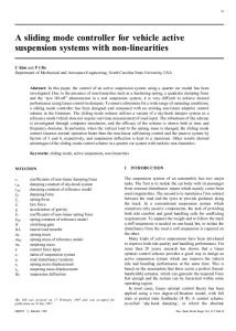
0 Fig. 1 . Two-link robot manipulator model.
where
IV. EXTENSION TO CARTESIAN SPACE CONTROL In this section, simular to [15] we extend the joint space sliding mode controller derived in the above section to the task space. To this effect, for a nonredundant manipulator, we simply replace the reference variable q, in (6) by
4,
= J-'(Zd - A ( z ~- 2))
(34)
and, accordingly
so that Let the equivalent parameter vector The same control law (8), (9), and (10) are then used again with (12) as the Lyapunov function. It can be easily verified that relation (1 1) is still valid. Following the same derivation as before, one obtain
17 5
=-
[ ~ q- zd + A Z ] ~ J - ~ ' K ~
x J-'[Jq - Zd
+A 4 < 0
(37)
+ AZ = 0.
(38)
Using the kinematic relation Z = J q , we recognize that expression (38) as the equation of sliding surface z AZ = 0, which in turn guarantees that Z + 0 as t + 03. Therefore, the previous sliding mode controller is globally stable and guarantees zero stead-state, Cartesian space, position error. Note from (34) and (35) that only the desired trajectories in Cartesian space Z d , i d , and x d have to be given. The quantities to be measured are joint positions q and joint velocities q. End-effector position z and velocity Z can be obtained from the direct kinematics, and therefore do not need to be explicitly measured. Also, note that the inverse Jacobian J-' appears in (34) and (35), and therefore singularity points should be avoided.
be
+ m2)r1
01
= (ml
ffg
= mgr;
03
= rri2i-1~2.
Therefore, the regressor matrix @ ( q ,q, 4,. q r ) defined in (7) is
which implies convergence to
Jq -id
(Y
ail
= 61,
a12
= Ulr
+e +
COS(9)
1'27
= 24'1, cos(d)
+
-
+ i z r cos(4) -
Oil7.sin(4)
(4+ $)4zr sin(4) + e cos(8 + Q)
@21
=0
@22
= a12
a23
= O i l , . sin(9)
+
cos( 0)
+ e cos(8 + 4 )
where e = g/r1, and g is the acceleration of gravity. The desired joint trajectory is given by 8d
= ~d = -90"
+ 52.5(1 -
CO5
1.26 t ) .
The goal of sliding mode control is to force the trajectory error = @ - @ d and 5 2 = Q - d d to sliding along the sliding surface which is chosen as &I
V. SIMULATION EXAMPLE The model chosen for simulation is a two-link planar manipulator as shown in Fig. 1. The dynamic equation is given by
s1
= Us&1
sg
= USf2
+ c1 + e2
where u s = 4. The resulting sliding mode equations are two decoupled first-order systems
et = - U S E z ,
i = 1,2.
IEEE TRANSACTIONS ON ROBOTICS AND AUTOMATION, VOL. 9, NO. 2, APRIL 1993
212
w a t a d . ) 10-3 180.00 160.00 140.00 120.00 100.00 80.00
0.40
60.00
0.20 40.00 0.00 20.00
-20.00 O.O0
3 I
I
I
0.00
2.00
4.00
-0.20 0.00
2.00
4.00
T(Sec.)
Fig. 5.
Sliding surface
52.
Fig. 2. Tracking error of joint one.
wad.)10-3 350.00
14.00 12.00 10.00 8.00
250.00
6.00 4.00 2.00 0.00 -2.00 4.00 -6.00
50.00
r---
0.00
--Lc-J
1
-8.00 -''.MI
I
--
8 T(Sec.)
0.00
2.00
4.00
Fig. 6 . Torque at joint one
we took 7j,(O) (i=1,2,3) in adaptation law (IO) as 700.00
'
7 j i ( O ) = 0.8, ljz(0) = 0.2 i j s ( 0 ) = 0.2.
600.00 500.00 400.00 300.00 200.00 100.00
I 0.00
I
I
2.00
4.00
Fig. 4. Sliding surface
In this simulation the control gains ~ d ( l i d=
lid
SI.
are selected as
T(Sec.1
Using control laws (8), (9), and (IO), Figs. 2 and 3 show the tracking errors. Figs. 4 and 5 show the sliding surfaces which confirm that adaptive sliding mode controller achieves its objective after an initial adaptation period. Figs. 6 and 7 show torques developed at the manipulator joints which result in undesirable control chattering. To test the robustness of the controller, a 0.5kg load was added to the joint 2. Changes in the load were not accounted for in the controller. Figs. 8 and 9 show the joint tracking errors with the load attached. It is confirmed that the validity of the proposed algorithm is explicitly for the purpose of the trajectory trackmg in the such uncertainty as handling a variable payload. To reduce the chattering, we implement the boundary layer controller given in (29), (30), and (31). Here the boundary layer is taken as 91 = 0 2 = 0.05. Figs. 10 and 11 show the tracking errors. Figs. 12 and 13 show sliding sectors. Figs. 14 and 15 show torques exerted at the manipulator. As can be seen from these figures, chattering is eliminated.
adl) = 8
rl = 0.2, r2 = 0.1.5, r3 = 0.1. The initial displacements and velocities are chosen as O(0) = 80", d ( 0 ) = 70": e(0) = d ( 0 ) = 0.
VI. CONCLUSION A sliding mode control scheme with the bound estimation is presented by using the theory of VSS. The major contribution of this methodology lies in the use of a special matrix, named regressor,
~
213
IEEE TRANSACTIONS ON ROBOTICS AND AUTOMATION, VOL. 9, NO. 2, APRIL 1993
Anslew.)x
10-3
180.00 160.00 140.00 120.00 100.00 80.00 60.00 40.00 20.00
-;::lEEE
0.00
\
-20.00
-12.00
40.00
-14.00 0.00
2.00
4.00
T(Sec.)
1 ,v/
'
0.00
2.00
4.00
T(Sec.1
Fig. 10. Tracking error of joint one with boundary layer.
Fig. 7. Torgue at joint two.
~ngle(~ad.)10-3 180.00
350.00
160.00 140.00
300.00
120.00 250.00
100.00
'
80.00 200.00
60.00 40.00
150.00
20.00 0.00
100.00
\
-20.00 40.00 -60.00 0.00
-80.00 0.00
2.00
4.00
T(Sec.1
I
I
I
0.00
2.00
4.00
Fig. 11. Tracking error of joint two with boundary layer.
Fig. 8. Tracking error of joint one with load.
10-3
~ngle(~ad.)10-3 350.00
700.00 600.00 500.00
250.00
400.00 300.00 150.00 200.00 100.00
100.00
0.00
-100.00
-0.00
I
I
0.00
2.00
I
-200.00
T(Sec.)
4.00
0.00
2.00
4.00
Fig. 9. Tracking error of joint two with load
Fig. 12. Sliding variable s i l .
which makes it possible for isolating the unknown parameters from the robotic dynamics. Based on the upper bounds of those unknown parameters which are estimated by a simple adaptive law, the proposed VSS controller guarantees the stability of the closed-loop
system. The robustness analysis shows that in the presence of the uncertainties, which are assumed to be unbounded and fast-varying, the closed-loop system can still be stabilized. Chattering is reduced by using the boundary layer technique. Simulation results show the validity of the proposed algorithm.
IEEE TRANSACTIONS ON ROBOTICS AND AUTOMATION, VOL. 9, NO. 2, APRIL 1993
214
REFERENCES
1.40 1.30 1.20 1.10 1 .OO
0.90 0.80
0.70 0.60
0.50
0.40 0.30 0.20
0.10
0.00
2.00
4.00
Fig. 13. Sliding variable sm2.
12.00
10.00 8.00
-
/
\\
/
6.00
4.00 2.00 0.00 -2.00 4.00 -6.00 -8.00 -10.00 0.00
2.00
4.00
Fig. 14. Torque at joint one with boundary layer.
3.00 2.00 1.00 0.00 -1.00 -2.00
-3.00 4.00 -5.00 -6.00 -7.00
-8.00 -9.00 -10.00 -11.00 -12.00 -13.00 0.00
2.00
4.00
Fig. 15. Torque at joint two with boundary layer.
ACKNOWLEDGMENT The authors are grateful to the Associate Editor, Professor Luh, and the reviewers for their encouraging and helpful comments.
[ l ] K. D. Young, “Controller design for a manipulator using theory of variable structure system,” IEEE Trans. Syst., Man, Cybern., vol. 8, pp. 101-109, 1978. 121 J. J. E. Slotine and S. S. Sastry, “Tracking control of nonlinear system using sliding surface, with application to robot manipulators,” Int. J. Contr., vol. 38, pp. 465492, 1983. [3] F. Harashima, H. Hashimoto, and K. Maruyama, “Practical robust control of robot arm using variable structure system,” in Pmc. lnt. Con$ Robotics Automat., 1986, pp. 532-539. [4] E. Bailey and A. Arapostathis, “Simple sliding mode control scheme applied to robot manipulator,” lnt. J. Contr., vol. 45, pp. 1197-1209, 1987. (51 B. E. Paden and S. S. Sastry, “A calculus for computing Filippov’s differential inclusion with application to variable structure control of robot manipulators,” IEEE Trans. Circuits Syst., vol. 34, pp. 73-82, 1987. [6] K. S. Yeung and Y. P. Chen, “A new controller design for manipulators using the theory of variable structure systems,” IEEE Trans. Automat. Contr., vol. 33, pp. 2 W 2 0 6 , 1988. [7] T. P. Leung, Q. J. Zhou, and C. Y. Su, “Practical trajectory control of robot manipulator using adaptive sliding control scheme,” in Proc. IEEE Con$ Decision and Contr., 1989, pp. 2647-2651. [SI S. W. Wijesoma and R. J. Richards, “Robust trajectory following of robot using computed torque structure with VSS,” Int. J. Contr., vol. 52, pp. 935-962, 1990. [9] C. Y. Su, T. P. Leung and Q. J. Zhou, “A novel variable structure control scheme for robot trajectory control,” in Proc. RAC 11th Triennial World Congress, 1990, vol. 5, pp. 117-120. [lo] L. C. Fu and T. L. Liao, “Globally stable robust tracking of nonlinear system using variable structure control and with application to a robotic manipulator,” IEEE Trans. Automat. Contr., vol. 35, pp. 1345-1350, 1990. [ l l ] H. L. Pei and Q. J. Zhou, “Variable structure control of linearizable systems with applications to robot manipulator,” in Proc. IEEE Int. Con$ Robotics Automat., 1991. [I21 T. P. Leung, Q. J. Zhou, and C. Y. Su, “An adaptive variable structure model following control design for robot manipulators,” IEEE Trans. Automat. Contr., vol. 36, pp, 347-353, 1991. [I31 V. I. Utkin, “Variable structure systems-Present and future,” Automat. and Remote Contr., vol. 44, pp. 1105-1 120, 1983. [I41 J. J. Craig, P. Hsu, and S. S. Sastry, “Adaptive control of mechanical manipulators,” in Proc. IEEE Int. Con$ Robotics Automat., 1986. [I51 J. J. E. Slotine and W. Li, “On the adaptive control of robot manipulators,” lnt J. Robotics Res., vol. 6, pp. 49-57, 1987. [I61 D. S. Koditschek, “Natural motion of robot arm,”in Proc. IEEE Cant Decision and Contr., 1984. [I71 F. Esfandiari and H. K. Khalil, “Stability analysis of continuous implementation of variable structure control,’’ IEEE Trans. Automat. Contr.. vol. 36, pp. 616-620, 1991. [18] W. Hahn, Stabilily of Motion. Berlin: Springer-Verlag, 1967. [I91 R. Ortega and M.W. Spong, “Adaptive motion control of rigid robots: A tutorial,” in Proc. IEEE Con$ Decision and Contr., 1988, pp. 1575-1584. 1201 J. J. E. Slotine and J. A. Coetsee, “Adaptive sliding controller synthesis for non-linear systems,” lnt. J. Contr., vol. 43, pp. 1631-1651, 1986.