(SLAM) problem asks if it is possible for an autonomous ve- hicle to start in an
unknown ... per proves that a solution to the SLAM problem is indeed possible.
1
A Solution to the Simultaneous Localisation and Map Building (SLAM) Problem M.W.M.G. Dissanayake, P.Newman, S. Clark, H.F. Durrant-Whyte and M. Csorba Australian Centre for Field Robotics Department of Mechanical and Mechatronic Engineering The University of Sydney NSW 2006, Australia Abstract— The simultaneous localisation and map building (SLAM) problem asks if it is possible for an autonomous vehicle to start in an unknown location in an unknown environment and then to incrementally build a map of this environment while simultaneously using this map to compute absolute vehicle location. Starting from the estimation-theoretic foundations of this problem developed in [1], [2], [3], this paper proves that a solution to the SLAM problem is indeed possible. The underlying structure of the SLAM problem is first elucidated. A proof that the estimated map converges monotonically to a relative map with zero uncertainty is then developed. It is then shown that the absolute accuracy of the map and the vehicle location reach a lower bound defined only by the initial vehicle uncertainty. Together, these results show that it is possible for an autonomous vehicle to start in an unknown location in an unknown environment and, using relative observations only, incrementally build a perfect map of the world and to compute simultaneously a bounded estimate of vehicle location. This paper also describes a substantial implementation of the SLAM algorithm on a vehicle operating in an outdoor environment using millimeter-wave (MMW) radar to provide relative map observations. This implementation is used to demonstrate how some key issues such as map management and data association can be handled in a practical environment. The results obtained are cross-compared with absolute locations of the map landmarks obtained by surveying. In conclusion, this paper discusses a number of key issues raised by the solution to the SLAM problem including sub-optimal map-building algorithms and map management.
I. Introduction The solution to the simultaneous localisation and map building (SLAM) problem is, in many respects, a “Holy Grail” of the autonomous vehicle research community. The ability to place an autonomous vehicle at an unknown location in an unknown environment and then have it build a map, using only relative observations of the environment, and then to use this map simultaneously to navigate would indeed make such a robot “autonomous”. Thus the main advantage of SLAM is that it eliminates the need for artificial infrastructures or a priori topological knowledge of the environment. A solution to the SLAM problem would be of inestimable value in a range of applications where absolute position or precise map information is unobtainable, including, amongst others, autonomous planetary exploration, subsea autonomous vehicles, autonomous air-borne vehicles, and autonomous all-terrain vehicles in tasks such
as mining and construction. The general SLAM problem has been the subject of substantial research since the inception of a robotics research community and indeed before this in areas such as manned vehicle navigation systems and geophysical surveying. A number of approaches have been proposed to address both the SLAM problem and also more simplified navigation problems where additional map or vehicle location information is made available. Broadly, these approaches adopt one of three main philosophies. The most popular of these is the estimation-theoretic or Kalmanfilter based approach. The popularity of this approach is due to two main factors. Firstly, it directly provides both a recursive solution to the navigation problem and a means of computing consistent estimates for the uncertainty in vehicle and map landmark locations on the basis of statistical models for vehicle motion and relative landmark observations. Secondly, a substantial corpus of method and experience has been developed in aerospace, maritime and other navigation applications, from which the autonomous vehicle community can draw. A second philosophy is to eschew the need for absolute position estimates and for precise measures of uncertainty and instead to employ more qualitative knowledge of the relative location of landmarks and vehicle to build maps and guide motion. This general philosophy has been developed by a number of different groups in a number of different ways; see ([4][5] and [6]). The qualitative approach to navigation and the general SLAM problem has many potential advantages over the estimation-theoretic methodology in terms of limiting the need for accurate models and the resulting computational requirements, and in its significant “anthropomorphic appeal”. The third, very broad philosophy, does away with the rigorous Kalman filter or statistical formalism while retaining an essentially numerical or computational approach to the navigation and SLAM problem. Such approaches include the use of iconic landmark matching ([7]), global map registration ([8]), bounded regions ([9]) and other measures to describe uncertainty. Notable are the work by Thrun et. al. [10] and Yamauchi et. al. [11]. Thrun et. al. use a bayesian approach to map building that does not assume Gaussian probability distributions as required by the Kalman filter. This technique while very effective for
2
localisation with respect to maps, does not lend itself to provide an incremental solution to SLAM where a map is gradually built as information is received from sensors. Yamauchi et. al. use a evidence grid approach that requires that the environment is decomposed to a number of cells. An estimation-theoretic or Kalman filter based approach to the SLAM problem is adopted in this paper. A major advantage of this approach is that it is possible to develop a complete proof of the various properties of the SLAM problem and to study systematically the evolution of the map and the uncertainty in the map and vehicle location. A proof of existence and convergence for a solution of the SLAM problem within a formal estimation-theoretic framework also encompasses the widest possible range of navigation problems and implies that solutions to the problem using other approaches are possible. The study of estimation-theoretic solutions to the SLAM problem within the robotics community has an interesting history. Initial work by Smith et al. [12] and DurrantWhyte [13] established a statistical basis for describing relationships between landmarks and manipulating geometric uncertainty. A key element of this work was to show that there must be a high degree of correlation between estimates of the location of different landmarks in a map and that indeed these correlations would grow to unity following successive observations. At the same time Ayache and Faugeras [14] and Chatila and Laumond [15] were undertaking early work in visual navigation of mobile robots using Kalman filter-type algorithms. These two strands of research had much in common and resulted soon after in the key paper by Smith, Self and Cheeseman [1]. This paper showed that as a mobile robot moves through an unknown environment taking relative observations of landmarks, the estimates of these landmarks are all necessarily correlated with each other because of the common error in estimated vehicle location. This paper was followed by a series of related work developing a number of aspects of the essential SLAM problem ( [2] and [3] for example). The main conclusion of this work was two fold. Firstly accounting for correlations between landmarks in a map is important if filter consistency is to be maintained. Secondly that a full SLAM solution requires that a state vector consisting of all states in the vehicle model and all states of every landmark in the map needs to be maintained and updated following each observation if a complete solution to the SLAM problem is required. The consequence of this in any real application is that the Kalman filter needs to employ a huge state vector (of order the number of landmarks maintained in the map) and is in general, computationally intractable. Crucially, this work did not look at the convergence properties of the map or its steady-state behaviour. Indeed, it was widely assumed at the time that the estimated map errors would not converge and would instead execute a random walk behaviour with unbounded error growth. Given the computational complexity of the SLAM problem and without knowledge of the convergence behaviour of the map, a series of approximations to the full SLAM solution were proposed which
assumed that the correlations between landmarks could be minimised or eliminated thus reducing the full filter to a series of decoupled landmark to vehicle filters (see Renken [16], ,Leonard and Durrant-Whyte [3] for example). Also for these reasons, theoretical work on the full estimationtheoretic SLAM problem largely ceased, with effort instead being expended in map-based navigation and alternative theoretical approaches to the SLAM problem. This paper starts from the original estimation-theoretic work of Smith, Self and Cheeseman. It assumes an autonomous vehicle (mobile robot) equipped with a sensor capable of making measurements of the location of landmark landmarks relative to the vehicle. The landmarks may be artificial or natural and it is assumed that the signal processing algorithms are available to detect these landmarks. The vehicle starts at an unknown location with no knowledge of the location of landmarks in the environment. As the vehicle moves through the environment (in a stochastic manner) it makes relative observations of the location of individual landmarks. This paper then proves the following three results: 1. The determinant of any submatrix of the map covariance matrix decreases monotonically as observations are successively made. 2. In the limit as the number of observations increases, the landmark estimates become fully correlated. 3. In the limit, the covariance associated with any single landmark location estimate is determined only by the initial covariance in the vehicle location estimate. These three results describe, in full, the convergence properties of the map and its steady state behaviour. In particular they show that • The entire structure of the SLAM problem critically depends on maintaining complete knowledge of the cross correlation between landmark estimates. Minimizing or ignoring cross correlations is precisely contrary to the structure of the problem. • As the vehicle progresses through the environment the errors in the estimates of any pair of landmarks become more and more correlated, and indeed never become less correlated. • In the limit, the errors in the estimates of any pair of landmarks becomes fully correlated. This means that given the exact location of any one landmark, the location of any other landmark in the map can also be determined with absolute certainty. • As the vehicle moves through the environment taking observations of individual landmarks, the error in the estimates of the relative location between different landmarks reduces monotonically to the point where the map of relative locations is known with absolute precision. • As the map converges in the above manner, the error in the absolute location of every landmark (and thus the whole map) reaches a lower bound determined only by the error that existed when the first observation was made. Thus a solution to the general SLAM problem exists and it is indeed possible to construct a perfectly accurate map and simultaneously compute vehicle position esti-
3
mates without any prior knowledge of vehicle or landmark locations. This paper makes three principal contributions to the solution of the SLAM. Firstly, it proves three key convergence properties of the full SLAM filter. Secondly, it elucidates the true structure of the SLAM problem and shows how this can be used in developing consistent SLAM algorithms. Finally, it demonstrates and evaluates the implementation of the full SLAM algorithm in an outdoor environment using a millimeter-wave radar sensor. Section 2 of this paper introduces the mathematical structure of the estimation-theoretic SLAM problem. Section 3 then proves and explains the three convergence results. Section 4 provides a practical demonstration of an implementation of the full SLAM algorithm in an outdoor environment using MMW radar to provide relative observations of landmarks. An algorithm addressing pertinent issues of map initialisation and management is also presented. The algorithm outputs are shown to exhibit the convergent properties derived in Section 3. Section 5 discusses the many remaining problems with obtaining a practical, large scale, solution to the SLAM problem including the development of sub-optimal solutions, map management and data association. II. The Estimation-Theoretic SLAM Problem This section establishes the mathematical framework employed in the study of the SLAM problem. This framework is identical in all respects to that used in Smith et. al. [1] and uses the same notation as that adopted in Leonard and Durrant-Whyte [3]. A. Vehicle and Land-Mark Models The setting for the SLAM problem is that of a vehicle with a known kinematic model, starting at an unknown location, moving through an environment containing a population of features or landmarks. The terms feature and landmark will be used synonymously. The vehicle is equipped with a sensor that can take measurements of the relative location between any individual landmark and the vehicle itself as shown in Figure 1. The absolute locations of the landmarks are not available. Without prejudice, a linear (synchronous) discrete-time model of the evolution of the vehicle and the observations of landmarks is adopted. Although vehicle motion and the observation of landmarks is almost always non-linear and asynchronous in any real navigation problem, the use of linear synchronous models does not affect the validity of the proofs in Section 3 other than to require the same linearisation assumptions as those normally employed in the development of an extended Kalman filter. Indeed, the implementation of the SLAM algorithm described in Section 4 uses nonlinear vehicle models and non-linear asynchronous observation models. The state of the system of interest consists of the position and orientation of the vehicle together with the position of all landmarks. The state of the vehicle at a time step k is denoted xv (k). The motion of the vehicle through the environment is modeled by a conventional lin-
Features and Landmarks Vehicle-Feature Relative Observation
pi Mobile Vehicle
xv
Global Reference Frame
Fig. 1. A vehicle taking relative measurements to environmental landmarks
ear discrete-time state transition equation or process model of the form xv (k + 1) = Fv (k)xv (k) + uv (k + 1) + vv (k + 1),
(1)
where Fv (k) is the state transition matrix, uv (k) a vector of control inputs, and vv (k) a vector of temporally uncorrelated process noise errors with zero mean and covariance Qv (k) (see [17] and [18] for further details). The location of the ith landmark is denoted pi . The “state transition equation” for the ith landmark is pi (k + 1) = pi (k) = pi ,
(2)
since landmarks are assumed stationary. Without loss of generality the number of landmarks in the environment is arbitrarily set at N . The vector of all N landmarks is denoted � �T . . . pT p = pT (3) 1 N where T denotes the transpose and is used both inside and outside the brackets to conserve space. The augmented state vector containing both the state of the vehicle and the state of all landmark locations is denoted � �T T . . . pT x(k) = xT . (4) v (k) p1 N The augmented state transition model for the complete system may now be written as Fv (k) 0 . . . xv (k) xv (k + 1) 0 0 p1 0 Ip 1 . . . p1 = .. . .. .. . .. .. . . . 0 pN pN 0 0 0 Ip N uv (k + 1) vv (k + 1) 0p1 0p1 + + .. .. . . 0pN
0pN (5)
x(k + 1) = F(k)x(k) + u(k + 1) + v(k + 1)
(6)
4
where Ipi is the dim(pi ) × dim(pi ) identity matrix and 0pi is the dim(pi ) null vector. The case in which landmarks pi are in stochastic motion may easily be accommodated in this framework. However, doing so offers little insight into the problem and furthermore the convergence properties presented by this paper do not hold.
The vehicle is equipped with a sensor that can obtain observations of the relative location of landmarks with respect to the vehicle. Again, without prejudice, observations are assumed to be linear and synchronous. The observation model for the ith landmark is written in the form (7) (8)
where wi (k) is a vector of temporally uncorrelated observation errors with zero mean and variance Ri (k). The term Hi is the observation matrix and relates the output of the sensor zi (k) to the state vector x(k) when observing the i( th) landmark. It is important to note that the observation model for the ith landmark is written in the form Hi = [−Hv , 0 · · · 0, Hpi , 0 · · · 0]
x ˆ(k + 1|k) = F(k)ˆ x(k|k) + u(k) x(k + 1|k) ˆ zi (k + 1|k) = Hi (k)ˆ
(10) (11)
P(k + 1|k) = F(k)P(k|k)FT (k) + Q(k),
(12)
respectively. Observation: Following the prediction, an observation zi (k + 1) of the ith landmark of the true state x(k + 1) is made according to Equation 7. Assuming correct landmark association, an innovation is calculated as follows •
B. The Observation Model
zi (k) = Hi x(k) + wi (k) = Hpi p − Hv xv (k) + wi (k)
k + 1 according to
(9)
This structure reflects the fact that the observations are “relative” between the vehicle and the landmark, often in the form of relative location, or relative range and bearing (see Section 4). C. The Estimation Process In the estimation-theoretic formulation of the SLAM problem, the Kalman filter is used to provide estimates of vehicle and landmark location. We briefly summarise the notation and main stages of this process as a necessary prelude to the developments in Sections 3 and 4 of this paper. Detailed descriptions may be found in [17],[18] and [3]. The Kalman filter recursively computes estimates for a state x(k) which is evolving according to the process model in Equation 5 and which is being observed according to the observation model in Equation 7. The Kalman filter computes an estimate which is equivalent to the conditional mean x ˆ(p|q) = E [x(p)|Zq ] (p ≥ q), where Zq is the sequence of observations taken up until time q. The error in the estimate is denoted x ˜(p|q) = x ˆ(p|q)−x(p). The Kalman filter also provides a recursive estimate of the co
T variance P(p|q) = E x ˜(p|q)˜ x(p|q) |Zq in the estimate x ˆ(p|q). The Kalman filter algorithm now proceeds recursively in three stages: • Prediction: Given that the models described in equations 5 and 7 hold, and that an estimate x ˆ(k|k) of the state x(k) at time k together with an estimate of the covariance P(k|k) exist, the algorithm first generates a prediction for the state estimate, the observation (relative to the ith landmark) and the state estimate covariance at time
νi (k + 1) = zi (k + 1) − ˆ zi (k + 1|k)
(13)
together with an associated innovation covariance matrix given by Si (k + 1) = Hi (k)P(k + 1|k)HT i (k) + Ri (k + 1). (14) • Update: The state estimate and corresponding state estimate covariance are then updated according to:
x ˆ(k + 1|k + 1) = x ˆ(k + 1|k) + Wi (k + 1)νi (k + 1) (15) P(k + 1|k + 1) = P(k + 1|k) − Wi (k + 1) × S(k + 1)WiT (k + 1)
(16)
Where the gain matrix Wi (k + 1) is given by −1 Wi (k + 1) = P(k + 1|k)HT i (k)Si (k + 1)
(17)
The update of the state estimate covariance matrix is of paramount importance to the SLAM problem. Understanding the structure and evolution of the state covariance matrix is the key component to this solution of the SLAM problem. III. Structure of the SLAM problem In this section proofs for the three key results underlying structure of the SLAM problem are provided. The implications of these results will also be examined in detail. The appendix provides a summary of the key properties of positive semi-definite matrices that are invoked implicitly in the following proofs. A. Convergence of the map covariance matrix The state covariance matrix may be written in block form as � Pvv (i|j) Pvm (i|j) P(i|j) = PTvm (i|j) Pmm (i|j), where Pvv (i|j) is the error covariance matrix associated with the vehicle state estimate, Pmm (i|j) is the map covariance matrix associated with the landmark state estimates, and Pvm (i|j) is the cross-covariance matrix between vehicle and landmark states. Theorem 1: The determinant of any submatrix of the map covariance matrix decreases monotonically as successive observations are made.
5
The algorithm is initialised using a positive semi-definite (psd ) state covariance matrix P(0|0). The matrices Q and Ri are both psd, and consequently the matrices P(k+1|k), Si (k+1), Wi (k+1)Si (k+1)WiT (k+1) and P(k+1|k+1) are all psd. From Equation 16, and for any landmark i, det P(k + 1|k + 1) = det[P(k + 1|k) − Wi (k + 1)Si (k + 1)WT (k + 1)] ≤ det P(k + 1|k) (18) The determinant of the state covariance matrix is a measure of the volume of the uncertainty ellipsoid associated with the state estimate. Equation 18 states that the total uncertainty of the state estimate does not increase during an update. Any principle submatrix of a psd matrix is also psd (see Appendix 1). Thus, from Equation 18 the map covariance matrix also has the property det Pmm (k + 1|k + 1) ≤ det Pmm (k + 1|k)
(19)
From Equation 12, the full state covariance prediction equation may be written in the form � Pvv (k + 1|k) Pvm (k + 1|k) = Y1 PTvm (k + 1|k) Pmm (k + 1|k)
As the number of observations taken tends to infinity a lower limit on the map covariance limit will be reached such that lim [Pmm (k + 1|k + 1)] = Pmm (k|k)
k→∞
Writing P(k + 1|k) as P� and P(k + 1|k + 1) as P⊕ for notational clarity, the SLAM algorithm update stage can be written as P⊕ = P� − Wi (k + 1)Si Wi T (k + 1) � = P� − P� Hi T S−1 i Hi P � � M1 −1 � = P� − Si M1 T M2 T M2 � T T M1 S−1 M1 S−1 i M1 i M2 = P� − T T M2 S−1 M2 S−1 i M1 i M2
� Fv Pvv (k|k)Fv T + Qvv PTvm (k|k)Fv T
T T � M1 = −P� vv Hv + Pvm Hpi T T � M2 = −P� vm Hv + Pmm Hpi
Thus, as landmarks are assumed stationary, no process noise is injected in to the predicted map states. Consequently, the map covariance matrix and any principle submatrix of the map covariance matrix has the property that Pmm (k + 1|k) = Pmm (k|k).
(20)
Note, that this is clearly not true for the full covariance matrix as process noise is injected in to the vehicle location predictions and so the prediction covariance grows during the prediction step. It follows from Equations 19 and 20 that the map covariance matrix has the property that det Pmm (k + 1|k + 1) ≤ det Pmm (k|k).
(24)
The update of the map covariance matrix Pmm can be written as T Pmm (k + 1|k + 1) = Pmm (k + 1|k) − M2 S−1 i M2 T = Pmm (k|k) − M2 S−1 i M2
Fv Pvm (k|k) . Pmm (k|k)
(21)
Furthermore, the general properties of psd matrices ensure that this inequality holds for any submatrix of the map covariance matrix. In particular, for any diagonal element 2 σii of the map covariance matrix (state variance), 2 2 σii (k + 1|k + 1) ≤ σii (k|k).
Thus the error in the estimate of the absolute location of every landmark also diminishes. Theorem 2: In the limit the landmark estimates become fully correlated
(23)
where
where Y1 =
(22)
(25)
T Equations 22 and 25 imply that the matrix M2 S−1 i M2 = −1 0. The inverse of the innovation covariance matrix Si is always p.s.d because the observation noise covariance Ri is psd, therefore Equation 22 requires that M2 = 0
Pmm (k|k)Hpi T = Pvm (k|k)Hv T
∀i
(26)
Equation 26 holds for all i and therefore the block columns of Pmm are linearly dependent. A consequence of this fact is that in the limit the determinant of the covariance matrix of a map containing more than one landmark tends to zero. lim [det Pmm (k|k)] = 0
k→∞
(27)
This implies that the landmarks become progressively more correlated as successive observations are made. In the limit then, given the exact location of one landmark the location of all other landmarks can be deduced with absolute certainty and the map is fully correlated. Consider the implications of Equation 26 upon the estimate d of the relative position between any two landmarks pi and pj of the same type. ˆi − p ˆj d=p = Gij x The covariance Pd of d is given by Pd = Gij PGij T = Pii + Pjj − Pij − Pij T
6
With similar landmarks types, Hpi = Hpj and so Equation 26 implies that the block columns of Pmm are identical. Furthermore, because Pmm is symmetric it follows that Pii = Pjj = Pij = Pij T
∀i, j
(28)
Therefore, in the limit, Pd = 0 and the relationship between the landmarks is known with complete certainty. It is important to note that this result does not mean that the determinants of the landmark covariance matrices tend to zero. In the limit the absolute location of landmarks may still be uncertain. Theorem 3: In the limit, the lower bound on the covariance matrix associated with any single landmark estimate is determined only by the initial covariance in the vehicle estimate P0v at the time of the first sighting of the first landmark. As described previously, the covariance of the landmark location estimates decrease as successive observations are made. The best estimates are obviously obtained when the covariance matrices of the vehicle process noise Q and the observation noise Ri are small. The limiting value and hence lower bound of the state covariance matrix can be obtained when the vehicle is stationery giving Q = 0. Under these circumstances it is convenient to use the information form of the Kalman filter to examine the behaviour of the state covariance matrix. Continuing with the single landmark environment,the state covariance matrix after this solitary landmark has been observed for k instances can be written as � T � � −Hv T P(k|k)−1 = P(k|k − 1)−1 + R1 −1 −Hv Hp1 T Hp1 (29) where because Q = 0, P(k|k − 1)−1 = P(k − 1|k − 1)−1 Using Equations 29 and as � P0v −1 −1 P(k|k) = 0
(30)
30 P(k|k)−1 can now be written 0 + Y2 0
(31)
where �
kHv T R1 −1 Hv Y2 = −kHp1 T R1 −1 Hv
−kHv T R1 −1 Hp1 kHp1 T R1 −1 Hpi
Invoking the matrix inversion lemma for partitioned matrices,
−1 T T P H P H 0v 0v v p1 P(k|k) = T −1 −1 H−1 H P H H P H H + Y v 0v v 0v p1 v 3 p1 p1 (32) where � −1 �T H−1 p1 R1 Hp1 . Y3 = k
Examination of the lower right block matrix of equation 32 shows how the landmark uncertainty estimate stems only from the initial vehicle uncertainty P0v . To find the lower bound on the state covariance matrix and in turn the landmark uncertainty the number of observations of the landmark is allowed to tend to infinity to yield in the limit
−1 T T P0v P0v Hv Hp1 lim P(k|k) = T k→∞ −1 −1 Hp1 Hv P0v H−1 H P H H v 0v v p1 p1 (33) Equation 33 gives the lower bound of the solitary landmark T −1 state estimate variance as H−1 p1 Hv P0v Hp1 Hv . Examine now the case of an environment containing N landmarks, The smallest achievable uncertainty in the estimate of the ith landmark when the landmark has been observed at the T −1 exclusion of all other landmarks is H−1 pi Hv P0v Hpi Hv . If more than one landmark is observed as k → ∞, as will be the case in any non-trivial navigation problem, then it is possible for the landmark uncertainty to be further reduced by theorem 1. In the limit the lower bound on the uncertainty in the ith landmark state is written as
� T −1 (34) Ppi ,pi ∞ = min H−1 pi Hv P0v Hpi Hv i∈[1,N ]
and is determined only by the initial covariance in the vehicle location estimate P0v . Note that because Q was set to zero in search of the lower bound the vehicle uncertainty remains unchanged at P0v as k → ∞. In the simple case where Hpi and Hv are identity matrices in the limit the certainty of each landmark estimate achieves a lower bound given by the initial uncertainty of the vehicle. When the process noise is not zero the two competing effects of loss of information content due to process noise and the increase in information content through observations, determine the limiting covariance. The problem is now analytically intractable, although the limiting covariance of the map can never be below the limit given by the above equation and will be a function of P0v , Q and R. It is important to note that the limit to the covariance applies because all the landmarks are observed and initialised solely from the observations made from the vehicle. The covariances of landmark estimates can not be further reduced by making additional observations to previously unknown landmarks. However, incorporation of external information, for example using an observation is made to a landmark whose location is available through external means such as GPS, will reduce the limiting covariance. In summary, the three theorems derived above describe, in full, the convergence properties of the map and its steady state behaviour. As the vehicle progresses through the environment the total uncertainty of the estimates of landmark locations reduces monotonically to the point where the map of relative locations is known with absolute precision. In the limit, errors in the estimates of any pair of landmarks become fully correlated. This means that given the exact location of any one landmark, the location
7
of any other landmark in the map can also be determined with absolute certainty. As the map converges in the above manner, the error in the absolute location estimate of every landmark (and thus the whole map) reaches a lower bound determined only by the error that existed when the first observation was made. Thus a solution to the general SLAM problem exists and it is indeed possible to construct a perfectly accurate map describing the relative location of landmarks and simultaneously compute vehicle position estimates without any prior knowledge of landmark or vehicle locations. IV. Implementation of the simultaneous localisation and map building algorithm This section describes a practical implementation of the simultaneous localisation and map building (SLAM) algorithm on a standard road vehicle. The vehicle is equipped with a millimeter-wave radar (MMWR) which provides observations of the location of landmarks with respect to the vehicle. The implementation is aimed at demonstrating key properties of the SLAM algorithm; convergence, consistency and boundedness of the map error. The implementation also serves to highlight a number of key properties of the SLAM algorithm and its practical development. In particular, the implementation shows how generally non-linear vehicle and observation models may be incorporated in the algorithm, how the issue of data association can be dealt with, and how landmarks are initialised and tracked as the algorithm proceeds. The implementation described here is, however, only a first step in the realisation and deployment of a fully autonomous SLAM navigation system. A number of substantive further issues in landmark extraction, data association, reduced computation and map management are discussed further in following sections.
Fig. 2. The test vehicle, showing mounting of the MMWR and GPS systems
A. Experimental setup
ronment that contains a number of radar reflectors. These reflectors appear as omni-directional point landmarks in the radar images. These, together with a number of natural landmark point targets, serve as the landmarks to be estimated by the SLAM algorithm. The vehicle is driven manually. Radar range and bearing measurements are logged together with encoder and steer information by an on-board computer system. In the evaluation of the SLAM algorithm, this information is employed without any a priori knowledge of landmark location to deduce estimates for both vehicle position and landmark locations. To evaluate the SLAM algorithm, it is necessary to have some idea of the true vehicle track and true landmark locations that can be compared with those estimated by the SLAM algorithm. For this reason the true landmark locations were accurately surveyed for comparison with the output of the map building algorithm. A second navigation algorithm, that employs knowledge of beacon locations is then run on the same data set as used to generate the map estimates (This algorithm is very similar to that described in [20].). This algorithm provides an accurate estimate of
Figure 2 shows the test vehicle; a conventional utility vehicle fitted with a MMWR wave radar system as the primary sensor used in the experiments. Encoders are fitted to the drive shaft to provide a measure of the vehicle speed and a Linear Variable Differential Transformer (LVDT) is fitted to the steering rack to provide a measure of vehicle heading. A differential GPS system and an inertial measurement unit are also fitted to the vehicle but are not used in the experiments described below. In the environment used for the experiments, DGPS was found to be prone to large errors due to the reflections caused by nearby large metal structures (usually known as ”multi-path” errors). The radar employed in the experiments is a 77 GHz FMCW unit. The radar beam is scanned 360 degrees in azimuth at a rate of 1-3Hz. After signal processing the radar provides an amplitude signal (power spectral density), corresponding to returns at different ranges, at angular increments of approximately 1.5o . This signal is thresholded to provide a measurement of range and bearing to a target. The radar employs a dual polarisation receiver so that even and odd bounce specularities can be distinguished. The radar is
capable of providing range measurements to 250m with a resolution of 10cm in range and 1.5o in bearing. A detailed description of the radar and its performance can be found in [19]. Figure 3 shows the test vehicle moving in an envi-
Fig. 3. Test vehicle at the test site. A radar point landmark can be seen in the left foreground
8
true vehicle location which can be used for comparison with the estimate generated from the SLAM algorithm. In the following, the vehicle state is defined by xv = [x, y, ϕ]T where x and y are the coordinates of the centre of the rear axle of the vehicle with respect to some global coordinate frame and ϕ is the orientation of the vehicle axis. The landmarks are modeled as point landmarks and represented by a cartesian pair such that pi = [xi , yi ], i = 1 . . . N. Both vehicle and landmark states are registered in the same frame of reference.
γ
p i(x i,y i)
ο
θi
ri
(x r,y r ) b
a ϕ
L
(x,y)
A.1 The process model Figure 4 shows a schematic diagram of the vehicle in the process of observing a landmark. The following kinematic equations can be used to predict the vehicle state from the steering γ and velocity inputs V ; x˙ = V cos(ϕ) y˙ = V sin(ϕ) ϕ˙ =
V tan(γ) , L
where L is the wheel-base length of the vehicle. These equations can be used to obtain a discrete-time vehicle process model in the form x(k) + ∆T V (k) cos(ϕ(k)) x(k + 1) y(k + 1) = y(k) + ∆T V (k) sin(ϕ(k)) (35) ϕ(k + 1) ϕ(k) + ∆T V (k)Ltan(γ(k)) for use in the prediction stage of the vehicle state estimator. The landmarks in the environment are assumed to be stationary point targets. The landmark process model is thus � � xi (k + 1) x (k) = i (36) yi (k + 1) yi (k) for all landmarks i = 1 . . . N . Together, equations 35 and 36 define the state transition matrix F(·) for the system. A.2 The observation model The millimeter wave radar used in the experiments returns the range ri (k) and bearing θi (k) to a landmark i. Referring to Figure 4, the observation model can be written as � ri (k) = (xi − xr (k))2 + (yi − yr (k))2 + wr (k) � � yi − yr (k) θi (k) = arctan (37) − ϕ(k) + wθ (k) xi − xr (k) where wr and wθ are the noise sequences associated with the range and bearing measurements, and [xr (k), yr (k)] is the location of the radar given, in global coordinates, by xr (k) = x(k) + a cos(ϕ(k)) − b sin(ϕ(k)) yr (k) = y(k) + a sin(ϕ(k)) + b cos(ϕ(k)) Equation 37 defines the observation model Hi (·) for a specific landmark.
Global Reference Frame
Fig. 4. Vehicle and observation kinematics
A.3 Estimation equations The theoretical developments in this paper employed only linear models of vehicle and landmark kinematics. This was necessary to develop the necessary proofs of convergence. However, the implementation described here requires the use of non-linear models of vehicle and landmark kinematics f (.) and non linear models of landmark observation h(.). Practically an Extended Kalman Filter (EKF) rather than a simple linear Kalman filter is employed to generate estimates. The EKF uses linearised kinematic and observation equations for generating state predictions. The use of the EKF in vehicle navigation and the necessary assumptions needed for successful operation is well known (see for example the development in [20]), and is thus not developed further here. A.4 Map initialisation and management In any SLAM algorithm the number and location of landmarks is not known a priori. Landmark locations must be initialised and inferred from observations alone. The radar receives reflections from many objects present in the environment but only the observations resulting from reflections from stationary point landmarks should be used in the estimation process. Figure 5 shows a typical test run and the locations that correspond to all the reflections received by the radar. Only about 30% of the radar observations corresponded to identifiable point landmarks in the environment. In addition to these, a large freight vehicle and a number of nearby buildings also reflect the radar beam and produced range and bearing observations. This data set illustrates the importance of correct landmark identification, initialisation and subsequent data association. In this implementation a simple measure of landmark quality is employed to initialise and track potential landmarks. Landmark quality implicitly tests whether the landmark behaves as a stationary point landmark. Range and bearing measurements which exhibit this behaviour are assigned a high quality measure and are incorporated as a landmark. Those that do not are rejected. The landmark quality algorithm is described in detail
9
100
locations are designated by stars. The actual (true) surveyed landmark locations are designated by circles. The vehicle path is shown with a solid line. In order to compute the “true” vehicle path, surveyed locations of the artificial point landmarks were used for running a map based estimation algorithm [20]. The absolute accuracy of the vehicle path obtained using this algorithm were computed to be approximately 5cm.
Radar Observations Vehicle Path Radar Refelectors
80
60
Y(m)
40
20
B.1 Vehicle localisation results
0
−20
Measured Feature Locations Estimated Feature Locations Vehicle Path
−40 −100
−50
0
50
40
X(m)
Fig. 5. A typical test run. Only 30% of radar observations correspond to identifiable landmarks Y(m)
in Appendix 2. The algorithm uses two landmark lists to record “tentative” and “confirmed” targets. A tentative landmark is initialised on receipt of a range and bearing measurement. A tentative target is promoted to a confirmed landmark when a sufficiently high quality measure is obtained. Once confirmed, the landmark is inserted into the augmented state vector to be estimated as part of the SLAM algorithm. The landmark state location and covariance is initialised from observation data obtained when the landmark is promoted to confirmed status. Figure 6 shows the computed landmark quality obtained at the end of the test run described in this paper.
30
20
10
0
−10 −40
−30
−20
−10
0
10
20
30
X(m)
Fig. 7. The “true” vehicle path together with surveyed (circles) and estimated (starred) landmark locations
Error in vehicle path (fixed features − slam) 0.6
Feature Quality
Error in X (m)
0.4 0 0
40
30
0 −0.2 −0.4 −0.6
0.8
0.79
0.75 20
−0.8 60 0.42 0
0
100
110
120
70
80
90 Time (sec)
100
110
120
0.5
0 0
0.85
0.77
0.69
90 Time (sec)
0.8
0.81
0.63
0.74
80
1
0
10
70
0
Error in Y (m)
Y (m)
0.2
0
−0.5
−10 −40
−30
−20
−10
0
10
20
30
X (m)
Fig. 6. Calculated landmark qualities at the end of the test run. Landmark quality ranges from 1 (for highest quality) to 0 (for lowest quality). Landmarks are marked with a star. Landmarks which are also circled are the artificial landmarks whose locations were surveyed so that the accuracy of the map building algorithm can be evaluated.
B. Experimental Results The vehicle starts at the origin, remaining stationary for approximately 30 seconds and then executing a series of loops at speeds up to 10m/s. Figure 7 shows the overall results of the SLAM algorithm. The estimated landmark
−1 60
Fig. 8. Actual error in vehicle location estimate in x and y (solid line), together with 95% confidence bounds (dotted lines) derived from estimated location errors. The reduction in the estimated location errors around 110 seconds is due to the vehicle slowing down and stopping.
The differences between the “true” vehicle path shown in Figure 7 and the path estimated from the SLAM algorithm are too small to be seen on the scale used in Figure 7. Figure 8 shows the error between true and SLAM estimated position in more detail. The figure shows the actual error in estimated vehicle location in both x and y as a function of time (the central solid line). The figure also shows
10
Innovation in range (m)
1.5
0 −0.5 −1 −1.5 30
40
50
60
70 80 Time (sec)
90
100
110
120
40
50
60
70 80 Time (sec)
90
100
110
120
Innovation in bearing (rad)
0.2
0.1
0
−0.1
−0.2 30
Fig. 9. Range and bearing innovations together with associated 95% confidence bounds Feature Number 1 0.5
0
−0.5 40
B.2 Map building results
50
60
70
80
90
100
110
80
90
100
110
Time (sec)
1.5
Error in Y (m)
1 0.5 0 −0.5 −1 −1.5 40
50
60
70 Time (sec)
Fig. 10. Difference between the actual and estimated location for landmark 1. The 95% confidence limit of the difference is shown by dotted lines Feature Number 3 3
Error in X (m)
2 1 0 −1 −2 −3 40
50
60
70
80
90
100
110
80
90
100
110
Time (sec)
1
0.5 Error in Y (m)
Figure 9 shows the innovations in range and bearing observations together with the estimated 95% confidence limits. The innovations are the only available measure for analysing on-line filter behaviour when true vehicle states are unavailable. The innovations here indicate that the filter and models employed are consistent. In addition to the ten radar reflectors placed in the environment, the map building algorithm recognises a further seven natural landmarks as suitable point landmarks. These can be seen in Figure 7 as stars (confirmed landmarks) without circles (without a survey location). Some of these natural landmarks correspond to the legs of a large cargo moving vehicle parked in the test site. The others do not correspond to any obvious identifiable point landmarks, but were recognised as landmarks simply because they returned consistent point-like radar reflections. The landmark qualities Q calculated at the end of the test run are shown in Figure 6. Figures 10 and 11 show the error between the actual and estimated landmark locations for two of the radar reflectors. One of these landmarks (landmark 1) was observed from the initial vehicle location at the start of the test run. The second landmark (landmark 3) was first observed about 30 seconds later into the run. Figures 10 and 11 also show the associated 95% confidence limits in the location estimates. As before, these are calculated using the estimated landmark location covariances. The landmark location estimates are thus consistent (and conservative) with actual landmark location errors being smaller than the estimated error. It can be seen that the initial variance of landmark 3 is much greater than that of landmark 1. This is due to the
1 0.5
Error in X (m)
95% (2σ) confidence limits in the estimate error. These confidence bounds are derived from the state estimate covariance matrix and represent the estimated vehicle error. The actual vehicle error is clearly bounded by the confidence limits of estimated vehicle error. The estimate produced by the SLAM algorithm is thus consistent (an indeed is conservative). The estimated vehicle error as defined by the confidence bounds does not diverge so the estimates produced are stable. The jump in x error near the start of the run is caused by the vehicle accelerating when the model implicitly assumes a constant velocity model. The slight oscillation in errors and estimated errors are due to the vehicle cornering and thus coupling long-travel with lateral errors. Selecting a suitable model for the vehicle motion requires giving consideration to the tradeoff between the filter accuracy and the model complexity. It is possible to improve the results obtained by assuming a constant acceleration model, and relaxing the non-holonomic constraint used in the derivation of the vehicle kinematic equation 35 by incorporating vehicle slip. This clearly increases the computational complexity of the algorithm. The SLAM algorithm thus generates vehicle location estimates which are consistent, stable and have bounded errors.
0
−0.5
−1 40
50
60
70 Time (sec)
Fig. 11. Difference between the actual and estimated location for landmark 3. The 95% confidence limit of the difference is shown by dotted lines
11
fact that the uncertainty in the vehicle location is small when landmark 1 is initialised, whereas landmark 3 is initialised while the vehicle is in motion and uncertainty in vehicle location is relatively high. These figures also show that there is some bias in the landmark location estimates. However, this bias is well within the accuracy of the true measurement (estimated to be ±0.1 m). Figures 12 and 13 show the estimated standard deviations in x and y of all landmark location estimates produced by the filter (for graphical purposes, the variances are set to zero until the landmark is confirmed). As predicted by theory, the estimated errors in landmark location decrease monotonically; and thus the overall error in the map reduces at each observation. Visually, the errors in landmark location estimates reach a common lower bound. As predicted by theory, this lower bound corresponds to the initial uncertainty in vehicle location. 2.5
Standard Deviation in X (m)
2
1.5
1
0.5
0 40
50
60
70
80
90
100
110
Time (sec)
Fig. 12. Decreasing uncertainty in landmark location estimates
3
Standard Deviation in Y (m)
2.5
2
1.5
1
0.5
0 40
50
60
70
80
90
100
110
Time (sec)
Fig. 13. Standard deviation of the landmark location estimate for all detected landmarks. As predicted, the uncertainty in landmark location estimates decrease monotonically
V. Discussion and Conclusions The main contribution of this paper is to demonstrate the existence of a non-divergent estimation theoretic solution to the SLAM problem and to elucidate upon the general structure of SLAM navigation algorithms. These contributions are founded on the three theoretical results proved in section 2; that uncertainty in the relative map estimates reduces monotonically, that these uncertainties converge to zero, and that the uncertainty in vehicle and absolute map locations achieves a lower bound. Propagation of the full map covariance matrix is essential to the solution of the SLAM problem. It is the crosscorrelations in this map covariance matrix which maintain knowledge of the relative relationships between landmark location estimates and which in turn underpin the exhibited convergence properties. Omission of these cross correlations destroys the whole structure of the SLAM problem and results in inconsistent and divergent solutions to the map building problem. However, the use of the full map covariance matrix at each step in the map building problem causes substantial computational problems. As the number of landmarks N increases, the computation required at each step increases as N 2 , and required map storage increases as N 2 . As the range over which it is desired to operate a SLAM algorithm increases (and thus the number of landmarks increases), it will become essential to develop a computationally tractable version of the SLAM map building algorithm which maintains the properties of being consistent and non-divergent. There are currently two approaches to this problem; the first uses bounded approximations to the estimation of correlations between landmarks, the second method exploits the structure of the SLAM problem to transform the map building process into a computationally simpler estimation problem. Bounded approximation methods use algorithms which make worst-case assumptions about correlatedness between two estimates. These include the covariance intersect method [21], and the bounded region method [22]. These algorithms result in SLAM methods which have constant time update rules (independent of the number of landmarks in the map), and which are statistically consistent. However, the conservative nature of these algorithms means that observation information is not fully exploited and consequently convergence rates for the SLAM method are often impracticably slow (and in some cases divergent). Transformation methods attempt to re-frame the map building problem in terms of alternate map or landmark representations which particularly have relative independence properties. For example, it makes sense that landmarks which are distant from each other should have estimates that are relatively independent and so do not need to be considered in the same estimation problem. One example of a transformation method is the relative filter [23][24] which directly estimates the relative, rather than absolute, location of landmarks. The relative landmark location errors may be considered independent thus resulting in a map building algorithm which has constant time complexity re-
12
gardless of the number of landmarks. More generally, a number of approaches are being developed for constructing “local map” and embedding these in a map management process. Here, consistent (full filter) local maps are linked by conservative transformations between local maps to generate and maintain larger scale maps. This embodies the idea that local landmarks are more important to immediate navigation needs than distant landmarks, and that landmarks can naturally be grouped into localised sets. Such transformation methods can exploit relatively low degrees of correlation between landmark elements to generate relatively decoupled sub-maps. The advantage of these transformation methods is that they highlight the real issue of large-scale map management. The theoretical results described in this paper are essential in developing and understanding these various approaches to map building. As discussed in the introduction there are a number of existing approaches to the localisation and map building problem. The important contribution of this paper is the proof that a solution exists. Furthermore it presents an algorithm that is efficient in the sense that it makes optimal use of the observations of relative location of landmarks for estimating landmark and vehicle locations, a property inherent in the Kalman filter. The value of all other alternative real-time SLAM algorithms that use similar information can be evaluated with respect to this “full” solution. This is particularly true in the case where simplifications are made to SLAM algorithms in order to increase the computational efficiency. The most effective algorithm for SLAM depends much on the operating environment. For example, the relative sparseness of occupied regions in the environment used for the example shown in section 4, the grid based approaches proposed in [11] and [10]. In an indoor environment the use of only point landmarks as in section 4 will be inefficient as the information such as the ranges to walls will not be utilised. The framework proposed in this paper, however, can incorporate geometric features such as lines (for example see [25]). In environments where geometric features are difficult to detect, for example in an underground mine, the proposed strategy will not be feasible. Many navigation systems used in outdoor environments relay on exogenous systems such as GPS. Clearly if external information is available these can be incorporated to the framework proposed in this paper. This is particularly useful in the situations where the exogenous sensor is unreliable, for example in case of GPS the errors such as those due to not being able to observe sufficient number of satellites or due to multipath errors caused when operating in cluttered environments. The implementation described in this paper is relatively small scale. It does, however, serve to illustrate a range of practical issues in landmark extraction, landmark initialisation, data association, maintenance and validation of the SLAM algorithm. The implementation and deployment of a large scale SLAM system, capable of vehicle localisation and map building over large areas will require both further development of these practical issues as well as a solution
to the map management problem. However, such a substantial deployment, would represent a major step forward in the development of autonomous vehicle systems. Appendix 1: Properties of positive semi-definite matrices 1. Diagonal entries of a psd matrix are non-negative 2. If A ∈ Rn×n is psd then for any matrix B ∈ Rn×m , BAB T is psd. 3. If A ∈ Rn×n and C ∈ Rn×n t are both psd then det(A+ C) ≥ det(A). 4. All principal submatrices of psd matrices are psd. 5. For A ∈ Rm×m , B ∈ Rn×m and C ∈ Rn×n , if � A B D= BT C is psd, then det(D) ≤ det(A) det(C) Appendix 2: Landmark Initialisation Algorithm The following describes the procedure used to initialise the landmark locations and associate observations to particular landmarks. This procedure also evaluates the quality of the landmarks. This algorithm is an essential precursor to the estimation process. It is not specific to the radar sensor but can be generalised to any sensor capable of observing landmarks in the environment. Two landmark lists are maintained. One list stores landmarks that are confirmed to be valid pi , i = 1 . . . N and the other stores potential landmarks yet to be validated qi , i = 1 . . . M. Initially both lists are empty. The map management algorithm proceeds as follows. 1. Given an observation [rf , θf ] at time instant k from the radar, the location of the landmark possibly responsible for this observation pf = [xf , yf ]T = g(x, y, ϕ, rf , θf ) and its covariance Pf is calculated using the following relationship. �
xf yf
� =
x(k) y(k)
� +
xvf (k) yvf (k)
where � � xvf (k) a cos(ϕ(k)) − b sin(ϕ(k)) + rf cos(ϕ(k) + θf ) = yvf (k) a sin(ϕ(k)) + b cos(ϕ(k)) + rf sin(ϕ(k) + θf ) and T + ∇grf θf R∇grTf θf Pf = ∇gxyϕ Pv ∇gxyϕ
where Pv is the covariance matrix of the vehicle location estimate extracted from the state covariance matrix P(k|k) and R is the measurement noise covariance. 2. An observation is associated with a landmark pi in the confirmed landmark set if df i = (pf − pi )T (Pf + Pi )−1 (pf − pi ) < dmin
13
where Pi is the covariance of the landmark location estimate pi , extracted from the state covariance matrix P(k|k). Note that df i is the Mahalanobis distance between pf and pi , and its probability distribution in this case is that of a χ2 variable with two degrees of freedom. Therefore, a suitable value for dmin can be selected such that the null hypothesis that pf and pi are the same is not rejected at some desired confidence level. Also if the above condition results in an observation being associated with more than one landmark p, the observation is rejected. If accepted, the observation is then used to generate a new state estimate. 3. If an observation cannot be associated with any confirmed landmark, then it is checked against the set of potential landmarks for possible association. Mahalanobis distance is again used as the criterion for association. If an association with the potential landmark qj is justified the new observation is used to update the location of the potential landmark qj and its covariance Pj . In addition, a counter cj indicating the number of associations with landmark qj is also incremented. 4. An observation that is not associated with either a confirmed or a potential landmark can be considered as a new landmark. In this case pf is added to the list of potential landmarks as qM+1 , a counter cM +1 is initialised and the number of the time step k is assigned to a timer tM +1 . 5. The potential landmark list qi , i = 1 . . . M is then examined against the following criteria. (a) If cj is greater than a predetermined number of associations cmin , the landmark j is considered to be sufficiently stable and therefore is transferred to the confirmed landmark list. (b) If (k − tj ) is greater than a predetermined tmax then the landmark j has not achieved the desired minimum number of associations over a sufficient length of time. Landmark j is therefore removed from the potential landmark list. 6. The probability density function (PDF) of the observations associated to a given landmark can be used to estimate its “quality”. As suggested in [26] the quality Qi of landmark i is calculated using the following equation. �l Qi =
1 j=1 2π
|Sj | �l
− 12
1 j=1 2π
T νj S−1 j νj ) 2 − 12
exp( |Sj |
References [1]
[2] [3] [4] [5] [6] [7] [8] [9]
[10]
[11] [12] [13] [14] [15] [16] [17] [18] [19] [20]
(38)
where l is the number of observations so far associated with the landmark i, where vj is the innovation of the observation j associated with landmark i observed at time k. Sj is the innovation covariance as defined by equation 14.The landmark quality Qi is the ratio between the sum of the probability densities of the observations and the maximum value of the probability density that is achieved when all the observations coincide with their predicted values. Therefore landmark qualities Q lie between 0 and 1. At reasonable intervals, landmark qualities can be calculated and landmarks that do not achieve a predetermined Qmin can be deleted from the map. 7. Return to step 2 when the next observation is received.
[21] [22] [23] [24]
[25]
[26]
R. Smith, M. Self, and P. Cheeseman, “Estimating uncertain spatial relationships in robotics,” in Autonomous Robot Vehicles, I.J.Coxand G.T. Wilfon, Ed., pp. 167–193. Springer Verlag, 1990. P. Moutarlier and R. Chatila, “Stochastic multisensor data fusion for mobile robot localization and environment modelling,” in Int. Symp. Robotics Research, 1989, pp. 85–94. J. Leonard and H. Durrant-Whyte, Directed Sonar Sensing for Mobile Robot Navigation, Kluwer Academic Publishers, 1992. Rodney A. Brooks, “Robust layered control system for a mobile robot,” in IEEE Journal Robotic Automation v RA-2 n p 14-23, 1986. Kuipers B.J. and Byun Y-T., “A robot exploration and mapping strategy based on semantic hierachy of spacial representation,” Journal of Robotics and Autonomous Systems 8: 47-63, 1991. T.S. Levitt and D.T. Lawton, “Qualitative navigation for mobile robots,” Artificial Intelligence Journal 44(3), pp. 305–360, 1990. Z.Zhang, “Iterative point matching for registration of free-form curves and surfaces,” International Journal of Computer Vision, 13(2):119-152, 1994. F. Cozman and E. Krotkov, “Automatic mountain detection and pose estimation for teleoperation of lunar rovers,” in Proc. IEEE Int. Conf. Robotics and Automation, 1997. U.D. Hanebeck and G. Schmidt, “Set theoretical localization of fast mobile robots using an angle measurement technique,” in Proc. IEEE Int. Conf. Robotics and Automation, Minneapolis, MN, April 1996, pp. 1387–1394. S. Thrun, D. Fox, and W. Burgard, “A probabilistic approach to concurrent mapping and localization for mobile robots,” Machine Learning 31, 29–53 and Autonomous Robots 5, 253–271, (joint issue), 1998. B. Yamauchi, A. Schultz, and W. Adams, “Mobile robot exploration and map building with continuous localization,” in ieeeicra, Leuven, Belgium, May 1998, pp. 3715 – 3720. R. Cheeseman P. Smith, “On the representation and estimation of spatial uncertainty,” Int. J. Robotics Research, 1986. H.F. Durrant-Whyte, “Uncertain geometry in robotics,” IEEE Trans. Robotics and Automation, vol. 4, no. 1, pp. 23–31, 1988. N. Ayache and O. Faugeras, “Maintaining a representation of the environment of a mobile robot,” in IEEE Trans. Robotics and Automation, 1989. R Chatila and Laumond J-P, “Position referencing and consistant world modelling for mobile robots,” in Proc. IEEE Int. Conf. Robotics and Automation, 1985. W.D. Renken, “Concurrent localisation and map building for mobile robots using ultrasonic sensors,” in Proc. IEEE Int. Conf. Itelligent Robots and Systems, 1993. Y. Bar-Shalom and T.E. Fortman, Tracking and Data Association, Academic Press, 1988. P. Maybeck, Stochastic Models, Estimation and Control, vol. 1, Academic Press, 1982. S. Clark and H.F. Durrant-Whyte, “Autonomous land vehicle navigation using millimeter wave radar,” in International Conference on Robotics and Automation, 1998. H. Durrant-Whyte, “An autonomous guided vehicle for cargo handling applications,” Internation Journal of Robotics Research, 15(5), pp. 407–440, 1996. J.K. Uhlmann, S.J. Julier, and M. Csorba, “Nondivergent simultaneous map building and localization using covariance intersection,” in SPIE, Orlando, FL, April 1997, pp. 2–11. M.Csorba, Simultaneous Localisation and Map Building, Ph.D. thesis, University of Oxford, Robotics Research Group, 1997. M. Csorba and H.F. Durrant-Whyte, “New approach to map building using relative position estimates,” in SPIE, Orlando, FL, April 1997, vol. 3087, pp. 115–125. P.M Newman, On The Solution to the Simultaneous Localisation and Map Building Problem, Ph.D. thesis, Dept Mechanical Engineering, Australian Centre For Field Robotics, University of Sydney, Sydney, Australia, March 1999. J.A. Castellanos, J.M.M. Montiel, J. Neira, and J.D. Tardos, “Sensor influence in the performance of simultaneous mobile robot localization and map building,” in Proc. 6th International Symposium on Experimental Robotics, Sydney, Australia, March 1999, pp. 203 – 212. D.Maksarov and H.F.Durrant-Whyte, “Mobile vehicle navigation in unknown environments: a multiple hypothesis ap-
14
proach.,” in IEE proceedings of Control Theory Application, Vol 142, No.4, July 1995.