A Space Vector PWM Method for Three-Level Flying-Capacitor Inverters M.A.Severo Mendes, Z. M. Assis Peixoto, P.F. Seixas, P.Donoso-Garcia Dept. of Electronics Engineering, Federal University of Minas Gerais AV. AntBnio Carlos, 6627, 31270-901 Belo Horizonte, MG, Brazil Email:
[email protected]
A.M.N. Lima Dept. of Electrical Engineering, Federal University of Paraiba Caixa Postal 10105, 58109-970 Campina Grande, PB, Brazil
Abstract-This paper presents a new space vector PWM method for a 3-level flying-capacitor inverter. In the proposed technique, boundary restrictions can be easily incorporated to minimize the harmonic distortion of the output voltages. Simple algebraic equations are used to calculate the pulse widths of the gate signals from the sampled reference voltages. This feature make easy the implementation in real time. The voltages on the flying capacitors are regulated by simple ON-OFF controllers independently of the output voltage control. The main features of the proposed technique are analyzed by computer simulations. The experimental tests obtained confirm the expected results.
E-
0 U
I
I
I
n
I. INTRODUCTION The increasing demand by quality and productivity in the industrial market requires continuous improvement of the voltage and current sources generated with power converters. The need for higher power ratings, reduction of harmonic distortion and EMI, led to the design of several multilevel power inverter topologies [8], [2], [8],[2], [3], [ 5 ] , [4],[6]. Among them the flying-capacitor inverter offers great advantages with respect to reduction in the number of semiconductor devices and possibility of independent control of output voltages and flying capacitors voltages.
Fig. 1. Simplified circuit diagram of a three-level Flying-Capacitor inverter
Table I shows the possible switching states for an inverter phase. Usually, the capacitor voltage e,,, x E { a , b , c } , is made equal to E / 2 . With this condition, the states A and B supply the same output voltage V,, = E/2. In the output voltage control the A and B states will indifferently be named 0 states. The variable c, ( t ) ,may assume the values 1, 0 or -1. TABLE I
SWITCHING STATES
This paper presents a new space vector PWM method for a 3-level flying-capacitor inverter [?I. In the proposed technique, boundary restrictions can be easily incorporated to minimize the harmonic distortion of the output voltages. Simple algebraic equations are used to calculate the pulse widths of the gate signals from the sampled reference voltages. This characteristic make easy the implementation in real time. The voltages on the flying capacitors are regulated by simple ON-OFF controllers independently of the output voltage control. The main features of the proposed technique are analyzed by computer simulations. The experimental tests obtained confirm the expected results.
FOR A THREE LEVEL INVERTER
ON B
N
-1
OFF
OFF
ON
ON
0
Figure 2 presents the current paths in the inverter for each state of the switches. In the P and N states, the load is directly connected to the DC bus and consequently these states do not affect the capacitor voltage. In the A and B states, the current of phase x flows through the capacitor C,. Considering the current sense indicated at figure 2, the capacitor will be charging in the A state and 11. THETHREE-LEVEL FLYING-CAPACITOR INVERTER discharging in the B state. The voltage e,, can then be controlled by appropriate selection of the 0 state. As the Figure 1 shows the simplified circuit diagram of a three- output voltage do not depend on the type of state used level GTO inverter. Each phase has four GTO switches, ( A or B ) , they can be used t o independently control the four freewheeling diodes and a capacitor. flying capacitor voltage.
0-7803-7067-8/01/$10.00 02001 IEEE
182
d N state
Fig. 2. Current paths in the inverter considering the four switching states .C
Fig. 4. Space voltage vectors of a three-level inverter
From table I and figure 2 can be verified that the number of power devices commutations during a change of switchings states depends on the initial and final states. In order to minimize the number of commutations the states change are classified in the form,
Good
{ NP
U +)
AorP ++ B Bud AorN H B
:
{ AP Hu BN
111. BASICEQUATIONS The output Phase voltage v z n ( t ) ,can be expressed in terms of the control variable c z ( t ) ,as follows:
-1
(1)
-1
The average value of the output phase voltages in the k-th switching period, V z n ( k ) , is calculated by:
A generic PWM signal using only good states commutations has been defined. This signal for a switching period fian ( k ) T is presented in figure 3. The time duration of the P, 0 and N states are indicated by ~ ~ , ( k ~) ,~ , ( and k) ~ ~ ~ ( k ) -1 -1 respectively. where, E,(k) is the average value of the control signal of phase x in the k-th period. From figure 3:
I
I
The average voltage vector in the k-th period, V d q ( k )is defined by:
Fig. 3. PWM Control signal c z ( t )
vdq(k)
2 = - (ean(k)
3
+ aebn(k)+ a2ecn(k))
(5)
with a= ej2a/3. Using the above equation and ( 3 ) it can be found that:
With four different switching states for each phase the three-level flying-capacitor inverter has 64 possible switching states. Figure 4 shows all the voltage vectors generated by the inverter of Fig. 1. These voltages vectors L 3 can be grouped into four different classes: (Z) zero vector Where C d q ( k ) is defined as the PWM control vector'of Vo having ten switching states; (S) small amplitude vecthe three-level inverter in the k-th period. Then, for a tors ( E / 3 ) having six different switching states each i.e., V I ,V d , V7, V ~ O , and (M) medium amplitude vec- given reference voltage vector Vgb(k) the PWM control tors (&E/3) having two switching states i.e., V3, v6, VS, vector can be determined by: V12, VISand VISand (L) large amplitude vectors ( 2 E / 3 ) 2 having only one switching state i.e., V2, V5, Vg, V ~ I V , 14 G ( k ) = EV,*,(k) (7) and V17. The zero sequence component of the PWM control vecUsually, in space vector methods, a voltage reference tor is defined by: vector is synthesized by the three closet voltage vectors of the inverter. This procedure reduces the harmonic content of the output voltages [l],[3].
183
~
The pulse widths T~~ and T~~ can be determined by using equations (7) and (8) and the inverse dq transformation. The pulse widths are calculated by:
In order to determine the pulse widths for a given phase the zero sequence component C o ( k ) must be selected. By a suitable choice of this component it is possible to minimize the harmonic distortion of the output voltages.
Iv.
DETERMINING PULSE
WIDTHS IN SECTOR
A
In order to simplify the study, the hexagon in Fig. 4 is divided into six sectors (A t o F). In this section, the switching patterns for sector A will be defined. These results can be easily extended to the others sectors. Fig. 5 shows a expanded view of sector A with its sub regions numbered from 1 to 4. All the possible switching states for each vector are also shown.
In the first switching period the complete switching pattern is employed. In the second period the switching pattern is mirrored minimizing the number of commutations. To reduce the load current ripple it is necessary t o split uniformly the utilization of the zero voltage vector over the switching period. With respect to Fig. 6 this is obtained if ~T"N = Too0 and 2Tppp = TOOO. The harmonic distortion of the output voltages can be minimized if the switching states corresponding t o the S vectors are equally used. With respect to Fig. 6 this is obtained if TPPO= TOONand TPOO= TONN. Using these restrictions and equation (9), a linear equation system is obtained:
NNN
000 --.
PPP
Fig. 5. Space voltage vectors in sector A
Solving this system gives the pulse widths that define the PWM control signals in Fig. 6 for reference voltage vectors inside sub region Al. The solution is given by:
A . Switching patterns f o r sub region A 1 The switching patterns consist in a ordered sequence of switching states corresponding t o the voltage vectors of the inverter in a given region. The ordering of the vectors can minimize the number of commutations of the inverter VI switches. The sub region A1 contains three vectors (VO, and V4) corresponding to seven different switching states. If the three vectors are employed in this sub region to form and ~ , , ( k ) is calculated by: the switching pattern the harmonic content of the output voltages is reduced. Such a pattern is named complete pattern. The complete switching pattern for sub region A1 is given by /PPP/PPO/POO/OOO/OON/ONN/NNN/. A similar procedure can be employed to determine the Fig. 6 shows the control signals of the three phases of the pulse widths for the sub regions A2 to A4. inverter for this switching pattern during two switching periods. Notice that in consecutive switching states only B. Overmodulation region The region extern to the hexagon of Fig.4 is usually one commutation occurs. A switching pattern that does not uses all the possible switching states is called reduced named overmodulation region. The reference voltage vectors in this region give rise to unrealizable pulse widths pattern.
184
~
TABLE I1
( ~ ( k) T ) . In this section, an algorithm is presented t o saturate the reference voltage vectors in the overmodulation region. In sector A, the limit of the overmodulation region is given by the condition (U:, - U:, 2 E ) as indicated in Fig.7. In the PWM method proposed, the reference voltage vector of coordinates (U:,, u f , U:%) in the overmodulation region is replaced by the voltage vector (U:,', U;,', U:,') with the same direction and the largest amplitude attainable by the inverter, as shown in Fig. 7.
LOCATIONOF
I
Sector
I
THE REFERENCE VOLTAGE VECTOR
Phase voltages order
1
I
!
I1 , - e k
eP
*
'VO
-
I
.
After the ordering procedure the phase voltages are referred as v;,(k), v;,(k) and u & ( k ) , where u;,(k) > uz,(k) > ugn(k). The pulse widths are then calculated using the same expressions employed for sector A replacing u:n(k), u i a ( k ) , and uFn(k) by U;n(k), G n ( k ) and U$n(k) respectively and similarly replacing T ~ , ,T p b , T ~T n~a , T,n b and T,, by ~ ~ rp2, 1 ,~ ~ T,I, 3 r,n 2 and 7,3 respectively.
I
3'
-
2.
d
VI. CONTROL OF THE
.
VI
v2
Fig. 7 . Overmodulation region
The voltage vector (U:,', U;,', U:,') is determined by the intersection of the line (U:, - U:, = E ) and the reference voltage vector (U:,, u f , U:,). Expressed in d,q coordinates:
FLYING
CAPACITORS VOLTAGES
The output voltages and flying capacitors voltages ( e c x ) can be controlled independently. The 0 states pulse widths given by equation 12 must be splited between the A and B states, as defined by equation 16.
The A and B states pulse widths are given by the value 5 p , ( k ) 2 -1, defined by:
of a control variable p z ( k ) , -1
The solution of this equation system in natural coordinates is:
Where, the factor k is given by:
In words, before entering the PWM algorithm, if an overmodulation condition is detected, the phase reference voltages must be scaled by a factor k , given by (15).
If px(k) = 1, only the state A is used, T,, ( k ) = T ~ (,k ) and Tbx ( k ) = 0. If px(k) = -1, Taz ( k ) = 0 and Tbz ( k ) = To, ( k ) . With px(k) = O,T,,(k) = T b x ( k ) . Figure 8 presents an ON/OFF controller for the flying capacitor voltage. The capacitor voltage and current information are used to determine the appropriate value for p , ( k ) . In fig. 8 diagram the variable p , ( k ) assume only the values f l . So, only one of the 0 states (A or B ) will be used in a given modulation period.
T H E RESULTS V . GENERALIZING
The determination of the pulse widths of the PWM control signals when the reference voltage vector is inside the sector A has been considered in the previous section. In this section these results are extended to the other sectors of Fig. 4. To determine the location of the reference voltage in the hexagon of Fig. 4 the reference phase voltages must be ordered. Table I1 shows the voltage ordering and respective vector locations.
Fig. 8. Block diagram of the on-off controller.
185
VII.
180
SIMULATION RESULTS
The proposed PWM method was tested in simulation with a three-level inverter supplying a three-phase RL load. The DC-link voltage is 300V and the load parameters are R = 5 0 and L = 5.5mH. The frequency of the reference voltage vector was 60Hz and the switching frequency equal to 1440Hz, corresponding to a frequency ratio (4)of 24. Fig. 9 shows the amplitude of the fundamental component of the output voltage when the modulation index (m) varies from 0 to 1. Linearity is observed up to m = 0.57 as expected. Fig. 10 shows the total harmonic distortion calculated by:
0'
I
0.01
0.02
Time
0.03 - (sec)
0.04
0.05
Fig. 12. Flying capacitor voltage - 20 V/div (E=300V)
VIII. EXPERIMENTAL RESULTS Fig. 11 shows the output line voltage for m = 0.5 and Fig. 12 shows the voltage at the flying capacitor.
A 3-level flying-capacitor inverter prototype was implemented to drive a three-phase induction motor of 2HP220/38OV. Flying capacitors of 47QpF/450V were used. The switching frequency was 1440Hz or 24 times the frequency of the reference signals. Figures 13 and 14 show the line voltage and line current waveforms respectively, for a modulation index of 0.5. The flying capacitor voltage under the same operation conditions is presented in figure 15, showing the effectiveness of the proposed control method.
Fig. 9. Fundamental component amplitude x modulation index
Fig. 13. Line output voltage - 100 V/div (E=300V) I
,
.
,
.
(
,
,
'0
01
0.2
03
0.4
0.5
06
0.7
modulation index - m
I oa
Fig. 10. SIG x modulation index
..
..
. .. . . , . .. . , . . .. . . . .
.
.
..
..
.
..
..
.
. . . .. . . . . .. . . . . .. . . . .. .
Fig. 14. Line output current
Fig. 11. Line voltage 100 V/div(f=60 Hz, m=0.5, q=24)
186
.
..
.. ..
.. ..
... ..
.
.
.
.
_I! .. ..
.. .
.
.
.
.
.
. ..
.. ..
;
;
{cbl;50 _................................................... ~
1
.. ..
= kv;,
.. .. . . ................................................ . . . . . . . . . .. . . .... . . ... . . . ... . . .... . . . .. . . . . . . . . . . ... . . .... .. .. .. .. .. .. .. .. . . . . . . . . . . . .. .. .. . . . . .. . . . . .. . . . .... . . . .... . . . . .. . . . . . . . . . . . . . . .. . . . ... . . . . . .. .. . . .. .. .. . . . . . . / . i v . . . / . . . . . . . . . . . . i. . . . .: . . . :
= kv;, v;, = Lugn U;,
(21)
5 - If vr,(k) - vgn(k) < E / 2 -+ region 1:
Fig. 15. Flying capacitor voltage - 5OV/div (E=300V)
Finally, figure 16 presents the harmonic analysis of the line voltage with a modulation index equal to 0.5.
>251i 200
Fig. 16. Harmonic spectrum of the Line voltage (m=0.5)
IX. CONCLUSION
8 -Else + region 3:
This paper presented a simple and useful PWM technique to control a three-level flying capacitor inverter. The pulse widths are calculated via simple algebraic equations, making the method appropriate to real time implementation. A simple method to control the flying capacitors voltages is employed. Complete independence between the output voltage control and flying-capacitor voltage control was assured. Low levels of capacitor voltage ripple and output voltages harmonic distortion were obtained. The experimental results indicated the validity of the proposed technique and the possibility of extending of the method to a greater number of levels.
REFERENCES Masato Koyama, Toshiyuki Fujii, Ryohei Uchida, and Taka0 Kawabata. Space voltage vector-based new pwm method for large capacity three-level gto inverter. In IEEE-IECON, volume 1, pages 271-276, November 1992. J.S. Lai and F. Peng. Multilevel converters - a new breed of power converters. In 30th IAS - Annual Meeting, volume 3, pages 2348-2356, October 1995. Yo-Han Lee, Bum-Seok Suh, and Dong-Seok Hyun. A novel pwm scheme for a three-level voltage source inverter with gto thyristors. IEEE Bansactions on Industry Applications, 32(2):260268, March/April 1996. M.A. Severo Mendes, P.F Seixas, P. Donoso-Garcia, and A.M.N Lima. An algebraic space vector pwm method for three-level voltage source inverters. In IEEE-IAS, CD-ROM-IAS2000, 2000. M.A. Severo Mendes, P.F Seixas, P. Donoso-Garcia, and A.M.N Lima. A new space vector pwm method for three-level voltage source inverters. In EPE-PEMC 2000, volume 3, pages 108-113, 2000. M.A. Severo Mendes, P.F Seixas, P. Donoso-Garcia, and A.M.N Lima. A space vector pwm method for three-level voltage source inverters. In IEEE-APEC, CDROM-APEC2000, 2000. T.A. Meynard and H. Foch. Multilevel conversion: High voltage chopper and voltage source inverters. In IEEE-PESC, pages 397-403, 1992. Akira Nabae, Isao Takahashi, and Hirofumi Akagi. A new neutral-point clamped pwm inverter. IEEE Transactions on Industry Applications, IA-17(5):518-523, september/october 1981.
X. APPENDIX- PWM ALGORITHM The complete algorithm for the proposed PWM method is described below.
Algorithm 1
- Sample the phase reference voltages: V;n
(IC) > v f ( k ) e
vFn ( k ) .
2 - Order the reference voltages samples, obtaining: v;n(k) 2 v2+n(k)2 v3*n(k) 3 - Use table I1 to determine the sector of the reference voltage vector. 4 - If v;,(k) - v z n ( k ) > E -+ overmodulation
187