A Sparse Signal Reconstruction Perspective for Source Localization ...

A Sparse Signal Reconstruction Perspective for Source Localization with Sensor Arrays by

Dmitry M. Malioutov B.S., Electrical and Computer Engineering Northeastern University, 2001

Submitted to the Department of Electrical Engineering and Computer Science in partial fulfillment of the requirements for the degree of Master of Science in Electrical Engineering and Computer Science at the

Massachusetts Institute of Technology July 2003 c 2003 Massachusetts Institute of Technology
All Rights Reserved.

Signature of Author: Department of Electrical Engineering and Computer Science July 29, 2003 Certified by: M¨ ujdat C ¸ etin Title: Research Scientist, Laboratory for Information and Decision Systems Thesis Supervisor Accepted by: Arthur C. Smith Chairman Department Committee on Graduate Students

2

A Sparse Signal Reconstruction Perspective for Source Localization with Sensor Arrays by Dmitry M. Malioutov Submitted to the Department of Electrical Engineering and Computer Science on July 29, 2003 in partial fulfillment of the requirements for the degree of Master of Science in Electrical Engineering and Computer Science

Abstract The theme for this thesis is the application of the inverse problem framework with sparsity-enforcing regularization to passive source localization in sensor array processing. The approach involves reformulating the problem in an optimization framework by using an overcomplete basis, and applying sparsifying regularization, thus focusing the signal energy to achieve excellent resolution. We develop numerical methods for enforcing sparsity by using
1 and
p regularization. We use the second order cone programming framework for
1 regularization, which allows efficient solutions using interior point methods. For the
p counterpart, the numerical solution is based on halfquadratic regularization. We propose several approaches of using multiple time samples of sensor outputs in synergy, and a method for the automatic choice of the regularization parameter. We conduct extensive numerical experiments analyzing the behavior of our approach and comparing it to existing source localization methods. This analysis demonstrates that our approach has important advantages such as superresolution, robustness to noise and limited data, robustness to correlation of the sources and lack of need for accurate initialization. The approach is also extended to allow self-calibration of sensor position errors by using a procedure similar in spirit to block-coordinate descent on an augmented objective function including both the locations of the sources and the positions of the sensors. The second direction of the work done in the thesis, which is intimately related to our approach for source localization, is theoretical analysis of the noiseless signal representation problem using overcomplete bases. Questions considered in this analysis include the uniqueness of solutions to the noiseless
0 problem, and the equivalence of solutions of the
0 ,
1 and
p problems. We consider an arbitrary overcomplete basis, and we show that under certain sparsity conditions on the underlying signal, such uniqueness and equivalence holds.

Thesis Supervisor: M¨ ujdat C ¸ etin Title: Research Scientist Laboratory for Information and Decision Systems

4

Acknowledgments Although my name appears as the sole author of the thesis, in reality a number of people are responsible for the work. First and foremost, I would like to thank my thesis advisor, Mujdat Cetin, and Alan Willsky, the leader of the Stochastic Systems Group. They introduced me to the topics of enforcing sparsity, regularization in inverse problems, and source localization, spent a good deal of time to make sure I understand the basic concepts, steered my research efforts to attack interesting and potentially solvable problems, and contributed many new ideas as the work progressed. I must thank Mujdat, and I encourage the reader to do so as well, for his titanic efforts in making my papers and my thesis readable, and teaching me the process of good scientific writing. Without his help I found myself on several occasions unable to understand my own writing which had been scribbled less than a week before. Working with Alan and Mujdat has been very inspiring: their energy, dedication, creative ideas, excellent organization, and the ability to be actively involved in and have a deep understanding of so many different research topics simultaneously, giving invaluable guidance to so many students on a weekly basis still does not fail to astonish me. I would also like to thank R. Moses, A. Baggeroer, A. Tsybakov, A. Samarov, M. Zatman, B. Sadler, and V. Stepanov for their discussions of my work and their suggestions for future directions, and improvements thereof. I would like to thank Jos Sturm for his help with SeDuMi, and for sending me patches to make it work for some of the optimization problems encountered in the thesis. I am very grateful to Peter Shor and Robin Blume-Kohout for their explanation of line packing in Euclidean spheres, and for providing me with a proof of the optimality of the regular simplex. Thanks to Brian Sadler for proposing a number of interesting directions for future work, and to Vladimir Stepanov for an interesting conversation on inverse problems. I have received a great deal of help from my fellow SSG students, which ranges from references to papers, explanation of obscure mathematical ideas, to tips for effective programming. Despite my sincere efforts, some outcomes from the last two years of interaction with this unique group of people did not get reflected in the thesis, but I feel they deserve to be mentioned anyway. I would like to thank my officemates Chen Lei, and Ayres Fan1 for teaching me the wonders of Mandarin subnormative lexicon, and perfecting my pronunciation; thanks to Jason Johnson for making me realize that I have a potential second career as a billiard hustler, and for introducing me to information geometry, and to structure estimation in graphical models. I have to thank Walter Wallstreet Sun for his sincere attempt to try to alleviate my ignorance in financial matters, for almost making me big money (more than a hundred dollars) in FOREX trading, 1

I found out recently that he also goes by J¯i Chaˇ o F` an, and also, to my great surprise, by Eros Fun.

5

6 and for stimulating mathematical conversations, especially on the subject of topology. Thanks to Eric Sudderth and Alex Ihler for taking the burden of running the network, and for their help and patience with computing troubles. Thanks to all the other SSG members and former members: Junmo Kim, Dewey Tucker, Andy Tsai (I never ate any of your God-forsaken candy because they tasted awful), Martin Wainwright, Patrick Kreidl, and Ron Dror. Also, despite all the harassment, humiliation, kicks and punches that I received from her, I’d like to thank Taylore Kelly. However, I have to warn her that she is yet to feel the full wrath of introducing me to PhotoShop. Tremble with fear Taylore, your fate is soon to come upon you! Finally, I would like to thank my friends and my family members for making me forget for brief periods of time about my work, my thesis, about MIT and its problem sets, and focus on fun-filled activities that range from learning how to cook and climb, to fixing a completely wrecked car, and measuring the speed of water in Tena river on a canoe. These moments made the past two years memorable and enjoyable.

Contents

1 Introduction 1.1 Overview of the problem addressed in the thesis . . . . . . . . . . . . . . 1.2 Outline and contributions . . . . . . . . . . . . . . . . . . . . . . . . . .

11 11 14

2 Introduction to Source Localization using Sensor Arrays 2.1 Observation model . . . . . . . . . . . . . . . . . . . . . . . 2.2 Methods for source localization . . . . . . . . . . . . . . . . 2.2.1 Classical beamforming . . . . . . . . . . . . . . . . . 2.2.2 Optimal beamforming: Capon’s method (MVDR) . 2.2.3 Subspace methods: MUSIC . . . . . . . . . . . . . . 2.2.4 Maximum Likelihood techniques . . . . . . . . . . . 2.2.5 Limitations of current methods . . . . . . . . . . . .

. . . . . . .

. . . . . . .

. . . . . . .

. . . . . . .

. . . . . . .

. . . . . . .

. . . . . . .

17 17 20 20 21 22 23 24

3 Introduction to Inverse Problems and Regularization 3.1 Ill-posed inverse problems and regularization . . . . . . 3.1.1 Quadratic regularization methods . . . . . . . . . 3.1.2 Non-quadratic regularization methods . . . . . . 3.2 Sparsity regularization . . . . . . . . . . . . . . . . . . .

. . . .

. . . .

. . . .

. . . .

. . . .

. . . .

. . . .

27 27 29 30 30

. . . . . . . . . . . . . . . . . . . . . . . . . . . . framework . . . . . . . . . . . . . . . . . . . . . . . . . . . . . . . . . . .

35 35 36 39 40 42 45 49 51 54 57

4
1 and
p Regularization 4.1
1 -regularization . . . . . . . . . . . . . . . . . . . . . 4.1.1 Noiseless case . . . . . . . . . . . . . . . . . . . 4.1.2 Handling noise . . . . . . . . . . . . . . . . . . 4.1.3 Second order cone programming . . . . . . . . 4.1.4 Representing
1 problems with complex data in 4.1.5 Numerical examples of
1 regularization . . . . 4.1.6 Analytical solution of a small problem . . . . . 4.1.7 Sign patterns of solutions, noiseless version . . 4.2
p Regularization . . . . . . . . . . . . . . . . . . . . . 4.2.1 Solution of positive definite linear systems . . .

. . . .

. . . .

. . . . . . . . . . . . SOC . . . . . . . . . . . . . . .

7

8

CONTENTS

5 Sparse-Regularization Framework for Source Localization 5.1 Narrowband problem . . . . . . . . . . . . . . . . . . . . . . . 5.1.1 Representation for one time sample . . . . . . . . . . . 5.1.2 Treating multiple time samples . . . . . . . . . . . . . 5.1.3 Treating each time index separately . . . . . . . . . . 5.1.4 Non-zero mean processing . . . . . . . . . . . . . . . . 5.1.5 Zero-mean beamspace processing . . . . . . . . . . . . 5.1.6 Joint-time inverse problem . . . . . . . . . . . . . . . 5.1.7 SVD-lp processing . . . . . . . . . . . . . . . . . . . . 5.1.8 Narrowband signals in the nearfield . . . . . . . . . . 5.2 Wideband scenario . . . . . . . . . . . . . . . . . . . . . . . . 5.2.1 Independent processing in each frequency band . . . . 5.2.2 Joint-frequency processing . . . . . . . . . . . . . . . . 5.2.3 Wideband focusing matrices . . . . . . . . . . . . . . . 5.3 Multi-resolution grid refinement and zooming . . . . . . . . . 5.4 Regularization parameter selection . . . . . . . . . . . . . . . 5.4.1 Discrepancy principle . . . . . . . . . . . . . . . . . . 5.4.2 Discrepancy principle in
1 constrained form . . . . .

. . . . . . . . . . . . . . . . .

. . . . . . . . . . . . . . . . .

. . . . . . . . . . . . . . . . .

. . . . . . . . . . . . . . . . .

. . . . . . . . . . . . . . . . .

. . . . . . . . . . . . . . . . .

6 Practical Issues and Performance Analysis 6.1 Details of the techniques and their implementation . 6.1.1 Effects of the grid . . . . . . . . . . . . . . . 6.1.2
p vs.
1 . . . . . . . . . . . . . . . . . . . . . 6.1.3 Initialization . . . . . . . . . . . . . . . . . . 6.1.4 Parameter selection . . . . . . . . . . . . . . 6.1.5 Number of resolvable sources . . . . . . . . . 6.2 Benefits of using the sparse regularization framework 6.2.1 Superresolution and robustness to noise . . . 6.2.2 Robustness to limited number of samples . . 6.2.3 Robustness to correlated sources . . . . . . . 6.2.4 Lack of need for accurate initialization . . . . 6.3 Bias . . . . . . . . . . . . . . . . . . . . . . . . . . . 6.4 Variance and the CRB . . . . . . . . . . . . . . . . .

. . . . . . . . . . . . .

. . . . . . . . . . . . .

. . . . . . . . . . . . .

. . . . . . . . . . . . .

. . . . . . . . . . . . .

83 . 84 . 84 . 85 . 86 . 88 . 90 . 92 . 92 . 94 . 96 . 96 . 97 . 103

. . . . . . . . . . . . .

. . . . . . . . . . . . .

. . . . . . . . . . . . .

. . . . . . . . . . . . .

. . . . . . . . . . . . .

59 60 60 62 62 63 64 65 68 72 73 73 75 76 77 79 80 80

7 Theoretical Analysis: solving the
0 problem by
p and related topics107 7.1
0 conditions . . . . . . . . . . . . . . . . . . . . . . . . . . . . . . . . . 108 7.1.1 Definition of rank-K unambiguity . . . . . . . . . . . . . . . . . 108 7.1.2 Uniqueness of
0 regularization . . . . . . . . . . . . . . . . . . . 109 7.1.3 Connection of rank-K unambiguity with maximum dot-product of columns of A . . . . . . . . . . . . . . . . . . . . . . . . . . . 110 7.1.4 Another condition for the uniqueness of
0 regularization . . . . 114 7.2 Solving the
0 problem by
1 . . . . . . . . . . . . . . . . . . . . . . . . 116 7.2.1 Sufficient condition for equivalence of
0 and
1 problems . . . . 117

9

CONTENTS

7.3

7.4

7.2.2 The insight into M (A) from the theory of spherical codes . 7.2.3 Sphere-packing bound . . . . . . . . . . . . . . . . . . . . . Conditions for the equivalence of
p and
0 problems . . . . . . . . 7.3.1 First condition for equivalence of
0 and
p for p ≤ 1 . . . . 7.3.2 Another equivalence condition for
p and
0 problems, p ≤ 1 Sparsity regularization: a sensitivity result for the noisy version. .

8 Model Errors and Self-Calibration 8.1 Self-calibration problem formulation . . . . . . . 8.2 Prior work in self-calibration . . . . . . . . . . . 8.3 Extension of our
1 /
p methods to self-calibration 8.4 Examples . . . . . . . . . . . . . . . . . . . . . .

. . . .

. . . .

. . . .

. . . .

. . . .

. . . .

. . . .

. . . .

. . . .

. . . .

. . . . . .

. . . .

. . . . . .

. . . .

. . . . . .

119 120 123 124 125 126

. . . .

129 130 131 132 134

9 Conclusion 137 9.1 Brief summary of the work in the thesis . . . . . . . . . . . . . . . . . . 137 9.2 Suggestions for further research . . . . . . . . . . . . . . . . . . . . . . . 138 A Estimation Theory Concepts and the Cramer Rao Bound

143

B Interior Point Methods

147

C Convex Analysis and Subdifferentials

151

D Conjugate Gradients (CG) and Preconditioning

153

E Minimizing
1 Norm subject to
∞ Constraint

155

F Analysis of the Applicability of Alternative Selection of the Regularization Parameter F.1 L-curve . . . . . . . . . . . . . . . . . . . . . F.2 Ordinary and Generalized Cross Validation . F.3 Universal and min-max rules . . . . . . . . .

Methods for Automatic 157 . . . . . . . . . . . . . . . 157 . . . . . . . . . . . . . . . 160 . . . . . . . . . . . . . . . 162

10

CONTENTS

Chapter 1

Introduction

In this thesis we consider the problem of sensor array source localization, and present a new approach based on a sparse signal representation perspective. The purpose of this chapter is to introduce the problem addressed in the thesis, motivate the need for a new approach, and describe our main contributions and the organization of the thesis.


1.1 Overview of the problem addressed in the thesis At the core of this thesis is the solution of the sensor array source localization problem by representing it as an inverse problem and imposing sparsifying regularization. Source localization using sensor arrays is a problem with many important practical applications including wireless communications [1, 2], radar [3, 4], sonar [5], and exploration seismology [6], among many others. The goal is to find the locations of the sources of wavefields which are impinging on an array of sensors. Practical applications require that the estimates of the locations be not only accurate under ideal conditions, but also robust to factors such as measurement noise, limitations in the amount of data, correlation of the sources, and modeling errors. For non-parametric methods, which result in a spatial energy spectrum, it is desired that the spectra have narrow peaks, low sidelobes, and the ability to localize sources even if they are within Rayleigh resolution of each other, i.e. the ability to achieve superresolution. Rayleigh resolution of an array depends on the number of sensors and on the spatial extent of the array, so it is possible to achieve any resolution simply by making larger arrays with more sensors. However, many practical applications have strict limits on the size of the array. One such application is surveillance using sensor networks. For example, suppose a large number of sensors are deployed into unknown terrain to monitor the activity in the area. Sensors are deployed over a large spatial extent, but power consumption limits severely the amount of communications that sensors can have, so source localization cannot be done coherently using all the sensors. Hence local groups of sensors have to provide accurate estimates of the locations of the objects of interest. These small arrays also have to be robust against noise, limited data, and modeling errors. In many source localization applications the physical dimensions of the sources of energy are small, or the sources are far enough from the array, so that they can be considered point sources. If, in addition, the number of sources is small, then the 11

12

CHAPTER 1. INTRODUCTION

spectrum of energy vs. location is sparse. Sparsity is a very valuable property to have. Many advanced source localization techniques for the localization of point-sources achieve superresolution by exploiting sparsity. For example, the key component of the MUSIC method [7] is the assumption of a small-dimensional signal subspace. We follow a different approach for exploiting such structure: we pose source localization as a linear inverse problem and use sparsity enforcing regularization. More specifically, our approach can be viewed as sparse representation of signals in terms of overcomplete bases. In this context, each basis vector corresponds to an array manifold vector for a possible source location among a sampling grid of locations. The representation of the observed sensor data in terms of an overcomplete basis is not unique, and we impose a penalty on lack of sparsity to regain uniqueness and, more importantly, to get sparse spectra. What penalties enforce sparsity? The ideal penalty to enforce sparsity is the count of nonzero elements of the resulting spectrum (which is sometimes referred to as the
0 -norm of the spectrum). However, the resulting problem is combinatorial in nature, and requires very heavy computational methods for its solution. We use related
1 norm and
p -norm penalties instead. The solution of a noiseless signal representation problem using
0 penalty has a close connection to solutions using
1 and
p penalties. In fact, under some assumptions on the number of sources, we show that in the noiseless case, the solution of these problems is the same for a general overcomplete basis. That means that if the signal of interest has a sparse enough representation in terms of an overcomplete basis, then, instead of using combinatorial optimization associated with
0 norms, we can find that sparse representation by imposing an
1 or an
p penalty, which leads to more tractable optimization problems. Prior work on this topic considered minimum
1 -norm representations in terms of a basis consisting of pairs of orthogonal bases [8, 9], and our work extends their results to arbitrary overcomplete bases. The results of equivalence of noiseless representations with minimum
0 ,
1 , and
p norms for sparse signals serve as a strong motivation for the use of
1 and
p penalties to enforce sparsity in the noisy case as well. The numerical solution of
1 -norm regularized linear inverse problems is much simpler that the solution of the
0 counterpart, since the
1 -norm penalty leads to convex objective functions. However, the solution is by no means trivial. The objective function is neither linear nor quadratic since we are dealing with
1 -norms of complex-valued data. We are led to consider second order cone programming (SOC) [10] which can be used to represent the resulting objective function, and also has an efficient procedure for solution through the use of interior point methods. The objective function corresponding to
p -norm regularization for p < 1 is a closer approximation to the objective function with
0 regularization, but, unlike the
1 objective function, it is non-convex1 . We can only expect to converge to local optima using smooth local optimization techniques. Global optimization methods are inherently computation-intensive, thus we do 1 For p < 1
p -norm is not a valid norm, (it does not satisfy the triangle inequality) but we choose to keep the same terminology for convenience.

13

Sec. 1.1. Overview of the problem addressed in the thesis

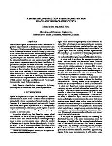
not use them. For local optimization of the objective function for
p -norm regularization we use an iterative half-quadratic method [11]. The representation of the source localization problem in the linear inverse problem form can be immediately used to solve single time sample problems. Unfortunately, there is limited information that can be extracted from a single time sample, and we are faced with the question of how to represent the multiple time sample source localization problem in our framework. In principle, we can represent the data for each of the multiple time samples in the linear inverse problem form and use sparsity enforcing regularization for each problem separately. Much better robustness to noise is achieved if we use multiple time samples in synergy. We look into several possibilities of joint use of multiple time samples. The one that appears the most promising is based on the singular value decomposition of the outputs of the sensors. We also consider additional practical problems, such as removing the effects of the grid, and automatically choosing the regularization parameter which balances the level of sparsity of the resulting spectrum versus the fidelity to the sensor measurements. 0 0

−10 Beamforming Capons MUSIC L1−SVD

Power (dB)

−20

−10

−20

−30 −30 Beamforming Capons MUSIC L1−SVD

−40 −40

−50 −50

−60

0

20

40

60

80

100

120

140

160

180

45

50

55

60

65

70

75

80

85

90

DOA (degrees)

(a)

(b)

Figure 1.1. (a) Comparison of beamforming, Capon’s, MUSIC, and
1 -SVD spectra for SNR=0 dB, and two sources coming from directions 60◦ and 65◦ with respect to the array axis.(b) Detail of (a).

To give a flavor of what we are able to do with our source localization technique, we present a simulation of an 8-sensor uniform linear array with 2 incoming narrowband farfield signals in Figure 1.1. The SNR is very low, 0 dB, and the sources are very close, the angular separation is 5◦ , so neither beamforming nor Capon’s method nor MUSIC are able to separate these two sources. However, one of the methods that we propose in the thesis,
1 -SVD has a clear separation between the two peaks in the spectrum. Also the sidelobes are nearly non-existent, which happens due to the fact that we explicitly optimized a measure related to sparsity! These results may look too good to be true, so we have to mention that the
1 -SVD technique is biased for closely spaced signals when the SNR is low. Nevertheless, small bias seems to be a good compromise for having excellent resolution and robustness to noise.

14

CHAPTER 1. INTRODUCTION

An additional concern that practical source localization methods have to handle is model errors, such as sensor position uncertainty. To that end we look into using a block-coordinate descent-like procedure on an extended cost function which takes into account both the locations of the sources and the positions of the sensors. The procedure alternates between two steps: the first step is source localization with estimated model parameters, and the second step is calibration of model parameters given the estimates of source locations from the previous step.


1.2 Outline and contributions Before describing the contents of the thesis chapter by chapter, we briefly summarize our main contributions. The first major contribution is the development of a sparse signal reconstruction framework for source localization. In this framework we formulate various optimization problems for single and multiple snapshot sensor data for the narrowband, wideband, farfield, and nearfield scenarios. We adapt and use two paradigms for the numerical solution of the optimization problems. Finally, we carry out an extensive performance analysis of the proposed source localization methods. The second contribution of the thesis is the extension of our source localization framework to perform self-calibration in the case of modeling errors. The third contribution is the development of conditions on the sparsity of the underlying signals that guarantee the uniqueness of solutions to the noiseless
0 sparse representation problem, and the equivalence of
0 ,
1 , and
p problems for a general overcomplete basis. Chapter 2: Introduction to Source Localization using Sensor Arrays

In this chapter we formulate the problem of source localization using an array of sensors. We describe several existing source localization methods. We end the chapter by describing some of the limitations of existing techniques thus motivating the need for our source localization framework. Chapter 3: Introduction to Inverse Problems and Regularization

We start by giving a brief overview of discrete ill-posed inverse problems, and motivate the need for regularization. We summarize the well-established quadratic regularization methods and discuss why they are inappropriate for the purpose of enforcing sparsity. Next we switch to non-quadratic regularization methods, an important subset of which is sparsity-enforcing regularization. Lastly, we describe an important linear inverse problem, sparse representation of signals using overcomplete bases. This problem serves a central role in the thesis: the basis of our work is the transformation of the source localization problem into the problem of sparse signal representation. Chapter 4:
1 and
p Regularization

In this chapter we describe numerical optimization of the objective functions corresponding to
1 and
p regularization. We start with the noiseless
1 signal represen-

Sec. 1.2. Outline and contributions

15

tation problem, and continue to several versions of noisy
1 problems. The data for source localization is complex-valued, and we are led to consider second order cone (SOC) programming for the numerical optimization of objective functions associated with
1 -norm penalization of complex quantities. We briefly summarize the SOC framework, and describe how to use it to represent our objective functions. In addition to showing numerical examples of
1 -regularization, we also solve a small problem analytically using non-smooth optimality conditions. We finish the
1 section by describing an interesting observation that we have made concerning sign patterns of exact solutions to the noiseless
1 problem. Next we describe
p regularization using an iterative half-quadratic procedure. Alternatively, it can be viewed as a quasi-Newton method with a positive definite Hessian approximation. The procedure relies on the conjugate gradients method for iterative solution of positive definite linear systems. Our main contribution in this chapter is the adaptation of the SOC framework for sparse complex signal representation with
1 regularization. In addition some theoretical analysis involving the analytic solution of a noisy
1 problem, and the observation of the existence of sign patterns of exact solutions, are also original. Chapter 5: Sparse-Regularization Framework for Source Localization

This chapter is the main contribution of the thesis. It describes the application of sparse regularization methodology from Chapter 4 to source localization using sensor arrays. We start by describing how to represent the nonlinear narrowband source localization problem with one time snapshot as a linear inverse problem. This problem can be viewed as signal representation using an overcomplete basis composed of a grid of samples from the array manifold. Next we present several approaches to use multiple time samples together in an efficient manner, and take a look at how to apply our framework to wideband source localization. Also, we develop an adaptive grid refinement procedure to get rid of the grid effects. An important issue in our framework is the choice of the regularization parameter. We describe a novel method for its automatic choice based on the discrepancy principle. In the course of our research we found that some previous work has been done with a similar flavor of enforcing sparsity for signal processing and even array processing applications, [12–14]. However, most of what we present has not been considered in these papers. Chapter 6: Practical Issues and Performance Analysis

This chapter is devoted to the analysis of the techniques developed in the previous chapter. First, we describe some details of the techniques and their implementation, such as the effects of the grid, comparison of
1 and
p , initialization, parameter selection, and the number of resolvable sources. Next we illustrate the benefits of using the sparse regularization framework for source localization. These include superresolution, robustness to SNR, to limited number of samples and to correlated sources, as well as no need for accurate initialization.

16

CHAPTER 1. INTRODUCTION

Finally, we analyze the bias, and compare the variance of our source localization methodology to the Cramer Rao Bound, as well as to the variances of existing source localization methods, using numerical simulations. Chapter 7: Theoretical Analysis: solving the
0 problem by
p and related topics

This chapter is another contribution of our thesis. We address theoretical analysis of uniqueness of solutions to the noiseless
0 regularization, and the equivalence of the noiseless
0 problems with noiseless
1 and
p problems. For the sake of generality, our analysis is separated from the array processing context, and presented in the context of signal representation using an overcomplete basis. This work was motivated by two papers [8] and [9], which consider the question of equivalence of
0 and
1 optimization for an overcomplete basis composed of two orthogonal bases. We extend their results to the general overcomplete basis case. In addition we prove some novel results: on the uniqueness of solutions of
0 problems using the notion of rank-K unambiguity, on the equivalence of
0 and
p problems for p < 1, and on sensitivity of noisy
1 regularization. Chapter 8: Model Errors and Self-Calibration

We motivate self-calibration of sensor arrays, briefly touch upon the observability conditions, and describe two existing methods based on block-coordinate descent. Next we use the same block-coordinate idea to extend our source localization framework to do self-calibration. This extension is also a contribution of the thesis. Chapter 9: Conclusion

This chapter summarizes the main ideas of the thesis and gives suggestions for further research in the area.

Chapter 2

Introduction to Source Localization using Sensor Arrays

The universal goal of array processing is to gather information from propagating waves. This nontrivial task is approached by sampling the spatiotemporal wavefield using an array of sensors. Some pieces of information that are commonly being sought about the wavefield include: the number and location of the sources of energy (or spatial energy spectrum), the signals generated by these sources, and the time evolution of all of the above. Using an array instead of a single sensor furnishes numerous benefits, comprising an improvement in signal to noise ratio, possibility of electronic steering and jamming suppression (instead of mechanical), and easier reconfiguration, among others. More importantly, source localization with omni-directional sensors is possible only when multiple sensors are available. Sensor array processing lends itself to many applications such as sonar, radar, exploration seismology and radio astronomy. Source localization is a branch of array processing which deals with determining the number and location of multiple sources using an array. In this chapter we formulate the source localization problem mathematically, provide an overview of most notable source localization methods, and describe some of their limitations as a motivation for our work.


2.1 Observation model Before we describe the conventional methods of source localization, it is necessary to present the mathematical model for the problem. For a more thorough covering of the material in this section the reader is referred to [15, 16]. Narrowband signal in the farfield of the array

We start with the most basic case, the localization of narrowband sources in the farfield of a uniform linear array. Let the uniform linear array in consideration consist of M omni-directional sensors with equal spacing d, residing on the x-coordinate axis. Taking the phase center of the array at the origin, the position of the m-th sensor is pm = (m − (M + 1)/2)d, m ∈ {1, .., M }. For the sources in the farfield of the array, 17

18

CHAPTER 2. INTRODUCTION TO SOURCE LOCALIZATION USING SENSOR ARRAYS

u (t)

u (t)

2

K

u1 (t)

... θ1

θ2

θK

...

... y (t) 1

y (t) d

2

...

y (t) i

...

y (t) M

Figure 2.1. An illustration of the geometry of source localization: sources uk (t), impinging on the array at angles θk producing sensor outputs ym (t).

the curvature of the wavefront is insignificant across the aperture of the array, and the plane wavefront approximation works very well. The solution of the wave equation with a single source generating signal f (t) has the form f (t − pT α), where p is the position, and α is the so called slowness vector aligned with the direction of propagation of the wave, and whose magnitude is equal to 1/c, the inverse of the propagation speed. The distance attenuation factor is not considered in the farfield model since it will be almost constant across the array if the sources indeed come from the farfield. The signal in the narrowband case can be expressed as u(t)exp(jω0 t), where u(t) is the baseband signal. It is modulated to frequency ω0 , which has to be much greater than the bandwidth of u(t) for the narrowband assumption to hold. In order to avoid spatial aliasing, sensor spacing has to be smaller than the half of the wavelength, d ≤ λ/2 = 2πc/(2ω0 ). Unless otherwise stated, we always take d = λ/2 for the narrowband case. The output of sensor m is ym (t) = u(t−τcenter )exp(j(ω0 (t−τcenter )−kT p)), where τcenter is the delay from the source to the phase-center of the array, and the wavenumber is given by k = ω0 α. Narrowband assumption allows us to ignore the delay between the sensors, kT p, in the baseband signal u(t); it is only present in the modulation. The complex envelope of the output of sensor m (i.e. the output after demodulation) can be written as ym (t) = u(t − τcenter )exp(−j(ω0 τcenter + kT p)). By measuring time relative to the phase center, the dependence on τcenter can be dropped. Thus, for a single source the complex envelope of the sensor outputs has the following form: y(t) = a(θ)u(t).

19

Sec. 2.1. Observation model

The manifold vector, a(θ) = exp(−jkT p) contains the phase delay information for the source coming from bearing θ with respect to the array axis. The parameterization of the manifold vector by θ can be done since kT pm = −(ω0 /c)(m − (M + 1)/2)dcos(θ). Due to the linearity of the system the superposition principle holds, and the model for K narrowband signals with the same center frequency can be written as y(t) = A(θ)u(t). The M × K matrix A(θ) is the manifold matrix containing the manifold vectors for different sources as its columns, A(θ) = [a(θ1 ), a(θ2 ), ..., a(θK )]. Sensor signal vector y(t) is a column vector whose m-th element is ym (t), and similarly u(t) is a column vector containing the signals uk (t) coming from all K sources. Vector θ contains source locations for all the K sources: θ = [θ1 , ..., θK ]T . Taking into account the inevitable presence of noise, and discretizing the waveforms, the final version of the model takes the following form:

y(t) = A(θ)u(t) + n(t),

t ∈ {1, .., T }

(2.1)

For simplicity, the noise is assumed to be spatially and temporally stationary and white, uncorrelated with the sources, and circularly symmetric. The covariance matrix takes the following form: E[n(t1 )nH (t2 )] = σ 2 I δ(t1 − t2 ), where δ() is the Kronecker delta function, and I is an identity matrix. The circular symmetry of the noise leads to E[n(t1 )nT (t2 )] = 0.

Nearfield of the array

The generalization of the model to the case where the sources lie in the nearfield of the model has a number of applications, for example audio speaker separation using a microphone array in enclosed spaces. The plane-wave approximation no longer holds, and the solution to the spherical wave equation at distance r from a single source f (t) is as follows: f (r, t) = (1/r)f (t − r/c). Again, considering the narrowband signal f (t) = u(t)exp(jω0 t), the complex envelope of the array output becomes ym (t) = (1/rm )u(t − rm /c)exp(−j(ω0 rm /c)). Here, rm is the distance from the source to the m-th sensor. Let rc be the distance from the source to the phase center of the array, and pm the position of m-th sensor. Taking into account the narrowband assumption, and shifting the time origin to correspond to the signal arriving at the phase center, the output can be rewritten as ym (t) = (1/rm )u(t)exp(−j(ω0 (rm − rc )/c)) = a(pm )u(t). The m-th component of the manifold vector, a(pm ) contains the phase and attenuation factors for the source arriving at sensor m. Using superposition, the model for K sources takes the exact same form as (2.1), except the columns of A(θ) contain the nearfield manifold vectors instead of the farfield ones. Unlike the farfield case, the response at the array depends not only on the bearings of the sources but also on their range, thus source localization furnishes both of these parameters.

20

CHAPTER 2. INTRODUCTION TO SOURCE LOCALIZATION USING SENSOR ARRAYS

Wideband signals

Finally, in the wideband case, the signal can no longer be well-approximated by a baseband signal modulated by a carrier. However, using the Fourier transform, a narrowband model can be written for each frequency: y(ω) = A(θ, ω)u(ω) + n(ω), ω ∈ {ω1 , .., ωW }

(2.2)

where y(ω) and u(ω) are Fourier transforms of y(t) and u(t) respectively. Note that in the narrowband case there is only one manifold matrix, whereas in the wideband case each frequency component ω yields a new manifold matrix, A(θ, ω). This happens since phase shift for a given delay depends on the frequency of the signal. To have multiple observations for each frequency, temporal data is usually divided into several blocks, and the Fourier transforms of each block are calculated. Or more generally, short-time Fourier transform, which allows the blocks to overlap, can be used. Second-order statistics

Most modern source localization methods rely on statistical characterization of the sensor outputs. The majority of them considers second-order statistics. The spatial covariance of the sensor outputs is R = E[y(t)yH (t)] = A(θ)PA(θ)H + σ 2 I, where the signal covariance matrix is P = E[u(t)uH (t)], and as discussed previously noise has a diagonal covariance: E[n(t)nH (t)] = σ 2 I. Many methods require that P is nonsingular, however situations in which this is not the case, e.g. due to the presence of multipath or coherent jamming, occur as well. Since the exact expectation is unknown, the standard 1
M ˆ sample covariance approximation is used: R = M t=1 y(t)yH (t). In the rest of this manuscript, we use R for both the actual and sample expectations, but the meaning of the symbol should be clear from context.


2.2 Methods for source localization
2.2.1 Classical beamforming The classical approach to source localization relies on scanning the power from different locations by steering the array. We discuss the farfield case1 . The array is steered by compensating the delays for the different sensor outputs by appropriately shifting the waveforms. When the weights on all the sensors are unity and no delays are introduced, the array is effectively steered at broadside (perpendicular to the array axis). For waves traveling in that direction, the delays for all the sensors are equal, and the delays with respect to the phase center are zero, requiring no compensation. Thus unity weighting produces constructive interference of the sensor outputs, and achieves the maximum power at broadside among all directions. Similarly, if the array is steered at an angle θ, the waveforms on the m-th sensor are advanced or delayed by −τm (θ), the negative of the delay relative to the phase 1

The nearfield case is analogous with the addition of a range parameter instead of just using bearing.

21

Sec. 2.2. Methods for source localization

center. The maximum power is achieved by steering at the direction from which the waves are arriving, assuming no aliasing is present. For the narrowband case the delays amount to phase shifts which can be implemented by complex weights w on the sensors. The array output thus becomes: z(t) = wH y(t) = wH a(θ)u(t). To steer the array to angle θ, the weights have to be set as w = a(θ). Due to the linearity of the system, the same approach is used to look for a superposition of plane-waves traveling from different directions, with identical carrier-frequencies. The beamforming spectrum can be represented as Pbf (θ) =

T 

wH (θ)y(t)22

(2.3)

t=1

Beamforming is a very simple and robust approach, which is widely used in practice. However, beamforming suffers from the Rayleigh resolution limit [15], which can be mitigated only by increasing the width of the array (the number of sensors): improving SNR or increasing observation time does not change resolution. The method parallels FIR time-series analysis. For example, to decrease the sidelobes levels, windowing can be used; however, no simple extensions are able to improve resolution. In the wideband case, the processing is usually done in frequency domain using short-time Fourier transforms. To work with wideband signals in the time domain, actual delays have to be implemented instead of phase shifts.


2.2.2 Optimal beamforming: Capon’s method (MVDR) The classical beamforming method has weights which are independent of the signals and noise. The idea of optimal beamforming is to use the estimated signal and noise parameters to improve the performance. One widely used method is Capon’s method, also called Minimum Variance Distortionless Response (MVDR), and Applebaum’s array [17]. It attempts to minimize the variance due to noise, while keeping the gain in the direction of steering equal to unity: wCAP (θ) = arg minw (E[wH yyH w]), subject to Re[wH a(θ)] = 1. The term variance is misleading: if the signals are random and zero-mean, then this is indeed the case, however, when the signals are non-random, wH Rw does not correspond to variance. Also, no attempt is made to separate the signal from the noise, so the aggregate energy is being minimized. The solution of this optimization problem can be shown to have the following form: wCAP (θ) =

R−1 a(θ) aH (θ)R−1 a(θ)

(2.4)

The source location estimate is obtained in the same way as for classical beamforming - simply by steering the array at a range of θ’s, and looking for maximum power. The resulting spectrum has an analytic expression: PCAP (θ) =

1 aH (θ)R−1 a(θ)

(2.5)

22

CHAPTER 2. INTRODUCTION TO SOURCE LOCALIZATION USING SENSOR ARRAYS

The main benefit of this method is a substantial increase in resolution compared with standard beamforming. In fact, as opposed to beamforming, the number of sensors does not impose a limit on resolution. With a non-degenerate array geometry (which avoids spatial aliasing), resolution increases without limit as SNR or the observation time are increased. An additional benefit is the lower amount of ripple in the sidelobes. However, the sidelobe level cannot go below σ 2 /M , the same value as for standard beamforming with unity weights. Some of the other shortcomings include an increase in the amount of computation compared to beamforming, poor performance with small amounts of time-samples (due to the difficulty of estimation of the sensordata covariance matrix) and inability to handle strongly correlated or coherent sources. Nevertheless, the combination of increased resolution, only moderate increase in computational complexity, and the robustness due to model errors which occur in practice (unlike some of the other conventional super-resolution methods) make this method one of the most widely used in practical applications. A more elaborate discussion of the method with motivations for all of the above assertions can be found in [15].


2.2.3 Subspace methods: MUSIC The MUSIC method [7] is the most prominent member of the family of eigen-expansion based source location estimators. The underlying idea is to separate the eigenspace of the covariance matrix of sensor outputs into the signal and noise components using the knowledge about the covariance of the noise. The sensor output correlation matrix admits the following decomposition: R = A(θ)PA(θ)H + σ 2 I = UΛUH =

(2.6)

H H 2 H Us Λs UH s + Un Λn Un = Us Λs Us + σ Un Un

(2.7)

Here, U and Λ form the eigenvalue decomposition of R, and Us , Un , Λs , and Λn = σ 2 IM −K are the partitions of the eigenspectrum into signal plus noise and signal subspaces. Provided that P is nonsingular, A(θ)PA(θ)H has rank K. The number of sources, K, has to be strictly less than the number of sensors, M , for the method to work. Hence, R has K eigenvalues which are due to the combined signal plus noise subspace, and M − K eigenvalues due to the noise subspace alone. Assuming that the noise has a flat spectrum of σ 2 , K eigenvalues corresponding to the signal and noise subspace are larger than the remaining M − K noise eigenvalues, which are equal to σ 2 . This information can be used to separate the two eigensubspaces. Due to the orthogonality of eigensubspaces corresponding to different eigenvalues for Hermitian matrices, the noise subspace is orthogonal to the steering vectors corresponding to the direction of propagation, thus UH n a(θ) = 0 for all directions from which the signals are impinging. MUSIC spectrum is obtained by putting the squared norm of this term into the denominator, which leads to very sharp estimates of the positions of the sources, (in the noiseless case the peaks of the spectrum approach infinity):

23

Sec. 2.2. Methods for source localization

PM U S (θ) =

1 aH (θ)Un UH n a(θ)

(2.8)

In contrast with the previously discussed techniques, MUSIC spectrum has no direct relation to power; it simply exhibits sharp peaks at the estimated source locations. Also, it cannot be used as a beamformer, since the spectrum is not obtained by steering the array. Unlike the the methods previously discussed, MUSIC provides a consistent (in the sense of estimation theory) estimate of the locations of the sources, as SNR and the number of sensors go to infinity. Despite the dramatic improvement in resolution, MUSIC suffers from a high sensitivity to model errors, such as sensor position uncertainty. Also, the resolution capabilities decrease when the signals are correlated. When some of the signals are coherent (perfectly correlated), the method fails to work. The computational complexity is dominated by the computation of the eigenexpansion of the covariance matrix. There are multiple extensions of MUSIC by using a weight matrix in the denominator, one of which is the Min-Norm algorithm [16]. Root-MUSIC [18] is a variant of MUSIC which instead of computing a spectrum, forms a polynomial using the noise subspace, and the source location estimates are the roots of the polynomial. RootMUSIC relies on the structure of the steering matrix for a uniform linear array (ULA), and cannot be extended to general arrays. The performance for ULAs is very similar to that of MUSIC, except for a somewhat higher robustness at limited numbers of time samples.


2.2.4 Maximum Likelihood techniques Maximum Likelihood (ML) methods [16,19] belong to the class of parametric methods. In contrast to the methods described above, the spectrum is not computed, but instead parameters of the model are estimated. A variety of methods resides under the ML header. One notable classification is in the assumed form of the signal. When the signals are modeled as deterministic, the method is called Deterministic ML (DML), when the signals are modeled as Gaussian, the method is called Stochastic ML (SML). Noise is usually modeled as stationary Gaussian. For deterministic maximum likelihood, the objective is to find θ, u(t), and σ 2 , to maximize the likelihood function: LDM L (θ, u(t), σ 2 ) =

T  (πσ 2 )−M exp(−y(t) − A(θ)u(t)22 /σ 2 ),

(2.9)

t=1

where θ is the vector of source locations. The log-likelihood is: lDM L (θ, u(t), σ 2 ) = −2M log σ +

T 1  (−y(t) − A(θ)u(t)22 ), σ2T t=1

(2.10)

24

CHAPTER 2. INTRODUCTION TO SOURCE LOCALIZATION USING SENSOR ARRAYS

Fortunately, it is not necessary to optimize over all the parameters, θ, u(t), and σ simultaneously, since once θ is known, we can use A(θ) to get explicit values for the other parameters: σ ˆ2 =

1 ˆ (t) = A(θ)† y(t) trace{Π⊥ A(θ)R} and u M

(2.11)

where A(θ)† is the pseudo-inverse of A(θ), and Π⊥ A(θ) is the projection matrix onto the orthogonal complement of the range space of A(θ). 2 The remaining unknown, the locations of the sources, can be found by minimizing the following cost function:

ˆ DM L = arg min θ θ

T 

2 ⊥ Π⊥ A(θ)y(t)2 = arg min trace{ΠA(θ)R}

t=1

θ

(2.12)

This cost function measures the sum of squares of projections of y(t) onto the orthogonal complement of the array manifold matrix, i.e. lack of fit of the range space of the manifold matrix to the data y(t). The optimization involves a K-dimensional search, where K is the number of impinging signals. K can be estimated using a variety of methods, such as Akaike information criterion (AIC) or minimum description length (MDL) [16, 20]. The computational complexity is considerably higher than for any of the methods described before. The benefits of ML family of methods is the ability to resolve coherent signals, ability to handle single snapshot scenarios, and better statistical properties [21]. A major problem with the ML-family of methods is the need for a very accurate starting point for the optimization procedure; otherwise the solution may converge to a local extremum.


2.2.5 Limitations of current methods Despite the existence of a multitude of various source localization methods we took the time to develop a new one. Part of the reason for such an undertaking is the desire to improve upon the performance of the existing methods; to that end we summarize some of their limitations. Beamforming is a very robust and simple source localization technique, but it has limited resolution. In Figure 2.2 we present two plots with beamforming spectra. We simulate a uniform linear array (ULA) with 8 sensors spaced at half-wavelength which is exposed to two farfield narrowband sources. In plot (a) the separation between the two sources is 20◦ , and beamforming is able to resolve the two sources. However once we move the sources closer together to 13◦ , within the Rayleigh resolution limit, the two peaks are merged, and the locations of the two sources cannot be determined. MUSIC and Capon’s methods go a long way to improve the resolution capabilities of beamforming. However, when the sources are close, and the SNR is low, they also 2

† A(θ)† = (A(θ)H A(θ))−1 A(θ)H , and Π⊥ A(θ) = I − A(θ)A(θ) , where I is an identity matrix.

25

Sec. 2.2. Methods for source localization 0

0

−5 −5

Power (dB)

Power (dB)

−10 −10

−15

−15

−20

−20

−25

−25

0

20

40

60

80

100

120

140

160

−30

180

0

20

40

60

80

100

120

140

160

180

DOA (degrees)

DOA (degrees)

(a)

(b)

Figure 2.2. Resolution limitations of beamforming. (a) Separation between the sources is 20◦ , peaks are resolved. (b) Separation between the sources is 13◦ , peaks are merged. 0

0 Capons MUSIC

Capons MUSIC

−5

−10

−5

−20

Power (dB)

Power (dB)

−15

−25

−30

−10

−15

−35

−40

−20

−45

−50

0

20

40

60

80

100

DOA (degrees)

(a)

120

140

160

180

−25

0

20

40

60

80

100

120

140

160

180

DOA (degrees)

(b)

Figure 2.3. Limitations of MUSIC and Capon’s methods (a) SNR=20 dB, separation between the sources is 10◦ , peaks are resolved by both MUSIC and Capon’s methods. (b) SNR=0 dB, separation between the sources is 5◦ , peaks are merged for both.

lose resolution and eventually are unable to separate the sources3 . Figure 2.3 illustrates what happens when we lower the SNR and bring the sources close together. In plot (a) SNR is 20 dB, and separation between the sources is 10◦ , so both MUSIC and Capon’s methods are able to resolve the two sources well. However, plot (b) shows that when SNR is decreased to 0 dB, and source separation is decreased to 5◦ , neither of the two methods can resolve the two sources. Some additional limitations of these two methods include inferior performance for correlated and coherent sources, and for scenarios with limited number of time samples. We present an in-depth comparison of these methods with our proposed source localization method in Chapter 6. 3

In fact every source localization technique has a lower limit on the SNR that it can withstand, but the method that we propose in the rest of the thesis has better robustness to low SNR than MUSIC and Capon’s methods.

26

CHAPTER 2. INTRODUCTION TO SOURCE LOCALIZATION USING SENSOR ARRAYS

Maximum Likelihood source localization techniques are parametric, so the result is not a spectrum but a set of point estimates of source locations. In general they are more robust than beamforming, MUSIC and Capon’s methods, but are computationally more demanding. Apart from computational complexity, the major drawback of ML source localization is the need for accurate initialization to insure convergence to global minima (instead of local ones). The method that we propose in this thesis does not suffer from the need for accurate initialization4 . A longer discussion of this issue appears in Chapter 6.

4

But, it does not decrease the computational cost of ML.

Chapter 3

Introduction to Inverse Problems and Regularization

We start this chapter by describing linear ill-posed inverse problems. Later in the thesis (in Chapter 5) we transform the source localization problem into this form. The solution of ill-posed inverse problems relies on regularization. Quadratic regularization is mentioned first. As we discuss, it is not well-suited for our goals, and we switch next to non-quadratic regularization and in particular sparsifying regularization. Sparsifying regularization is discussed in the context of signal representation using overcomplete bases, a special case of a linear ill-posed inverse problem. Our transformed source localization problem can be viewed as signal representation using overcomplete bases.


3.1 Ill-posed inverse problems and regularization In inverse problems [22–24] the function from the unknown quantity that we wish to find to the observations is known. The goal is to find a meaningful inverse function. Mathematically, we have y = T(x), where x ∈ X is the unknown and y ∈ Y is the vector of observations.1 Usually, T() is a well-behaved continuous operator, and the solution of the forward problem (find y given x) meets no significant obstacles. The inverse mapping from y to x in the problems of interest is much less friendly. The difficulties may include lack of solution, non-unique solutions, or a discontinuous dependence of the solution on the observations. The presence of any of these issues makes the problem ill-posed. As we stated it, the problem is too general, and we make additional assumptions that X and Y are finite-dimensional, and T is a linear operator: y = Tx, y ∈ CM , x ∈ CN , T ∈ CM ×N

(3.1)

Lack of solutions means that y does not lie in the range of T (T is not surjective), and lack of uniqueness means that the nullspace of T is not trivial (T is not injective). The standard approach to treat these two obstacles is by taking the Moore-Penrose 1

X and Y are Hilbert spaces, i.e. complete metric spaces with an inner product defined.

27

28

CHAPTER 3. INTRODUCTION TO INVERSE PROBLEMS AND REGULARIZATION

pseudo-inverse, T† . Consider the singular value decomposition (SVD): T = UΣV =

min(M,N )



ui σi vi

(3.2)

i=1

Let K = rank(T). Then the pseudo-inverse is defined as †

T =

K 

vi σi−1 ui

(3.3)

i=1

By applying the pseudo-inverse we find the minimum-norm least squares solution. If y = Tx, then the reconstruction is  ˆ = T† y =  x

K  j=1

 vj σj−1 uj  y

=

K  j=1

vj σj−1 uj

min (M,N )

ui σi vi x =

i=1

(M,N ) K min K N     σi    vj uj ui vi x = vi vi x = (IN − vi vi )x σj j=1

i=1

i=1

i=K+1

ˆ is Here IN is an N × N identity matrix. Whenever K < N , the reconstruction x only an approximation to x. The component of x that lies in the nullspace of T is set to zero (T† chooses the min-norm solution). Since T† is a linear function in a finite dimensional space, then it is necessarily continuous. However, in some applications the condition number of T† may be very large, making the pseudo-inverse discontinuous for all practical purposes. Now let us consider what happens when we add noise: y = Tx + n. Even the addition of small amount of noise to the
observations may render the solution completely useless: −1  ˆ+ K T† y = T† (Tx + n) = x i=1 vi σi ui n. The power distribution of projections of white noise on all the left singular vectors is uniform, (E[(ui n)2 ] is not a function of i). By applying the pseudo-inverse we are multiplying the noise components by inverses of σi , the last few of which are very large since T is ill-conditioned. The amplification of these noise components dominates the solution, and the signal component of interest becomes hidden under the noise floor. Much of the effort in the field of discrete illposed problems is directed at making good approximations to T† which are much less sensitive to noise. Regularization is used to solve ill-posed problems by incorporating apriori knowledge about x to stabilize the problem and to provide reasonable and useful solutions. For example, if it is known that the solution should be a discretization of a continuous function, this knowledge allows us to discard the wildest looking candidates, and to considerably reduce the set of possible solutions. The task is to minimize some measure J1 (x) of proximity of y to the range space of T, as well as to satisfy as much as possible

Sec. 3.1. Ill-posed inverse problems and regularization

29

the apriori information about x, by minimizing some appropriate measure J2 (x). The two objectives typically cannot be both minimized at the same time, so we need a compromise, which can be simply obtained by taking a linear combination of the two: J(x) = J1 (x) + λJ2 (x)

(3.4)

Scalar λ is the regularization parameter balancing the tradeoff between the fidelity to the data, J1 (x), and the fidelity to the prior information, J2 (x). There is a whole family of solutions indexed by λ, with the non-regularized (least squares) solution if λ = 0, and a solution strongly favoring the apriori information when λ is large. In general, choosing an appropriate λ is problem-dependent, and is a nontrivial task. With an appropriate choice for J(x), regularization effectively deals with all the three aspects of ill-posedness. Solution exists for any y ∈ Y, since we are allowing y outside the range of T with the use of J1 (x). Also, proper choice of J2 (x) deals with lack of uniqueness and can dramatically reduce sensitivity to noise (improve the Lipschitz constant of the inverse function), making it “continuous enough” for practical applications.


3.1.1 Quadratic regularization methods One of the most well-known approaches to regularization is due to Tikhonov [25]. Tikhonov’s method assumes that the norm of the solution should be small, which limits the amount of amplification due to small eigenvalues. The cost function takes the form J(x) = Tx − y22 + λx22

(3.5)

The
2 -norm of the residual is the data-fidelity term, J1 (x), and the term x22 serves as J2 (x) in (3.4). The Tikhonov cost function has a closed-form solution:  K   σi2 ui y ˆ= x vi (3.6) 2 σi + λ σi i=1

Other quadratic regularization methods, such as the truncated or damped SVD follow
ui y ˆ= K a similar pattern [26]: x i=1 wi σi vi . They can be regarded as weighted pseudo σi2 . inverses with weights wi . Tikhonov regularization is a special case with wi = σ2 +λ i The idea of all of these methods is to leave the large singular values almost unchanged, and to limit the effects of the inverses of small singular values. To incorporate other forms of prior information, the following generalization of the cost function can be used: J(x) = Tx − y22 + λL(x − x∗ )22 , where L is a linear operator most suitable for the prior of interest, and x∗ is an apriori estimate. The quadratic family of regularization methods is very suitable for many practical applications, and has the benefit of a closed-form solution, and tractable methods for choosing the regularization parameters. However, since the inverse operator is always a linear function of the data, there are limitations on what can be achieved. In particular, due to the linearity it is impossible to recover the part of x which belongs to the nullspace of T.

30

CHAPTER 3. INTRODUCTION TO INVERSE PROBLEMS AND REGULARIZATION


3.1.2 Non-quadratic regularization methods Using a quadratic form for both the data-fidelity and the prior term leads to a linear dependence of the reconstruction on the data. The most important benefit of linearity is the computational tractability of the problem. However, linearity also suffers from a salient drawback of irrecoverability of sharp features. This occurs due to the fact that forward operators T in most inverse problems of interest have a low-pass frequency response, and a smoothing effect. High-frequency components belong to the nullspace of T, and cannot be recovered by a linear inverse mapping. It has been shown both theoretically and practically that allowing for the more general non-linear form of regularization can lead to a dramatic improvement in this respect, preserving sharp edges and other strong features and leading to super-resolution in the reconstruction [26]. However, computational complexity increases considerably due to this generalization. That is particularly true for the case of non-convex functions. Two popular non-quadratic cost functions are total variation and entropy [26].
Total variation puts a penalty on the sum of variations of the signal J2 = Dx1 = |[Dx]i |, where D is a discrete approximation to the gradient operator. Total variation is most frequently used in image processing applications, such as image restoration. In comparison to the Tikhonov regularization with L = D, the penalty on strong features is less severe, and the reconstruction can contain sharp edges. It works very well in practice with images that can be described as piecewise-smooth.
Maximum entropy regularization uses an entropy-like prior term: J2 (x) = |xi |log(|xi |). Some variations are possible using cross-entropy, and divergence. Cost functions with this form lead to greater energy concentration in the reconstruction (most coefficients are very small, and a few are large). Another term for energy concentration is sparsity. This is most suitable for data which exhibit the same behavior, for example in spectrum estimation for signals with several harmonics, or point source localization. Another regularizing function which has the same sparsifying effect is the
1 -penalty: J2 = x1 . This is similar to the total-variation except we take the
1 -norm of the values of x instead of their derivatives. Total variation allows sparse jumps of the gradient of x, whereas the
1 penalty favors sparse values of x. To lower the penalty on strong features even further, several non-convex functions have also found use. The
p -quasi-norm with
p p p < 1, J2 = xp = i |xi | , produces even stronger energy concentration in the reconstruction. Strong energy-concentration property makes
1 and
p -regularization very suitable for the reconstruction of sparse signals, for example for those arising in array processing. We rely on
1 and
p penalization for the rest of the thesis. We discuss the benefits of sparsity in much greater detail in the next section, since it is the heart of our source localization methodology.


3.2 Sparsity regularization The selection of a proper regularizer intimately depends on the property of x that one wishes to enforce, and that depends on the particular application. In many mathe-

Sec. 3.2. Sparsity regularization

31

matical inverse problems, priors of choice are different forms of smoothness or energy constraints, and the corresponding regularizers are the
2 norms of x or its derivatives. Sparsity prior is useful when signals x that we look for have to be sparse. We define sparsity of a vector x by the presence of a small number of large elements and zeros elsewhere. An appropriate numerical measure of sparsity is the count of non-zero elements. An important linear inverse problem which has a good use for sparsity priors is the problem of signal representation using overcomplete bases. Our source localization framework, the subject of this manuscript, is built on such overcomplete representation ideas. The base for this discussion is the work of Mallat [27], Donoho [28], Rao [14] and others on function approximation and optimal basis selection. The problem of choosing an appropriate basis for a family of signals has received a great deal of attention over the past decade, and many new bases were introduced, such as wavelet bases, ridgelets, and curvelets, among many others [29]. Despite the fact that any minimal spanning basis for a finite-dimensional space can represent perfectly any signal in the space, when only a subset of possible signals is of interest, some bases have better representational properties than others. For example, using the Fourier basis for signals consisting of a few harmonics is more natural than using the standard basis. What do we mean by “more natural”? In this context that means that the representation is much sparser with the Fourier basis than with the standard basis. If the signal consists of harmonics with frequencies on the standard discrete Fourier grid, then the number of nonzero elements in the discrete Fourier transform is equal to the number of harmonics. However, using the standard basis, the number of nonzero elements is in general equal to the dimension of the space, which may be much greater than the number of harmonics. Some applications which benefit greatly from sparsity of representation are signal compression, denoising, and parameter estimation. In compression for information transmission, if the representation of the signal is not sparse then we need to transmit the whole signal. However, if under a change of basis the representation becomes sparse, then substantial savings are possible. Most coefficients of the representation are very small (by definition of sparsity) and if we set them to zero the perceptual quality of the signal will be affected very little. So we are left with transmitting only the large coefficients, which are few in number. This idea found use in commercial compression algorithms. For example, the JPEG2000 standard 2 uses the fact that the representation of natural images using Daubechies maxflat wavelet bases is considerably sparser than the original representation (in terms of the standard basis). Another application where sparsity plays a key role is denoising. If the signal is sparse then separating it from the noise requires considerably less effort than when signal power is evenly distributed along the support of the signal. Therefore, for the purpose of facility of denoising of a class of signals, it is worthwhile to find a basis in which the representation of all signals belonging to this class is as sparse as possible. The number of sparsely representable signals directly depends on the number of 2

See http://www.jpeg2000info.com for details.

32

CHAPTER 3. INTRODUCTION TO INVERSE PROBLEMS AND REGULARIZATION

elements in the signal dictionary. Every minimal basis has the same number of sparsely representable signals. In order to increase the number of signals with sparse representation, an overcomplete basis has to be used. Some overcomplete bases that have been considered include a concatenation of several orthogonal bases, e.g. standard and Fourier which can sparsely represent superpositions of continuous sinusoids and local sharp phenomena. Another possibility is to use a single extended non-orthogonal basis such as a Fourier basis with the number of considered frequencies exceeding the dimension of the space. The overcomplete Fourier basis allows to represent sparsely harmonics with frequencies in between the standard Fourier grid. By turning to an overcomplete basis we lose a very important property, the uniqueness of representation. To regain uniqueness, we search for the sparsest solution among the many possible solutions. Mathematically, when no noise is present the problem is as follows: given a signal y ∈ CM , and an overcomplete basis T ∈ CM ×N , we would like to find x ∈ CN such that y = Tx, and x is sparse. Define x00 to be the number of non-zero elements of x. We would like to find min x00 subject to y = Tx. This is a very hard combinatorial problem. In Chapter 7 we show 3 that under some conditions on T and x, the optimal value of this problem can be found exactly by solving a related problem: min xpp subject to y = Tx, where 0 < p ≤ 1 (we consider separately two cases, p = 1, and general p, 0 < p ≤ 1). A natural extension when we allow white Gaussian noise n is y = Tx + n,

(3.7)

min y − Tx22 + λxpp .

(3.8)

which can be solved by

If we let J1 (x) = y − Tx22 , and J2 (x) = xpp , then we have nothing but a regularized inverse problem of the form in (3.4). When p = 1 this method is called basis pursuit [29] (or LASSO [30] in the statistical literature). The prior term, J2 (x) has an effect of enforcing sparsity. Figure 3.1 gives some insight into why
p -regularization with p ≤ 1 favors sparse x. In plot (b), we show the level sets of
p norms to the p-th power (xpp ) for p = 0.5, p = 1, and p = 2 of a two-dimensional vector. For a fixed
2 -norm, i.e. for all vectors that lie on a circle with fixed radius,
p norms with p ≤ 1 are minimized on the coordinate axes, i.e. preferring that some of the coefficients are set exactly to zero, while others are large. In other words it prefers sparse solutions. This argument can be generalized to vectors in higher dimensions. Plot (a) shows
p norms for the same p’s in one dimension. It shows that the penalty on large features (large xi ) is less for smaller p. Strong features are penalized much less severely in
p penalization with p ≤ 1 than in
2 penalization (Tikhonov regularization). This motivates the smoothing effect of
2 -penalization, and the feature-preserving behavior of
p for p ≤ 1. 3

Our results extend the work of [8] and [9].

33

Sec. 3.2. Sparsity regularization 40

4

35

p=2

3.5

p=1

30

p=2 3

25

2

x2

|x|

p

2.5

p=1

p = 0.5

20

1.5

15 1

p = 0.5 10

0.5

0 −2

5 −1.5

−1

−0.5

0

0.5

1

1.5

2

x 5

10

15

20

25

30

35

40

x1

(a)

(b)

Figure 3.1. (a) 1-D Plot of
x
pp , p = 0.5, 1, 2. (b) 2-D Level sets of
x
pp , same p.

Another observation from Figure 3.1 is that
1 norm is convex, whereas when p < 1,
p -norm is no longer convex4 . The computational complexity for the minimization of some non-convex cost functions (
p in particular) can be ameliorated by using the halfquadratic regularization method [31]. The key idea is to introduce a supplementary vector s, and an extended cost function, Q(x, s) which is quadratic in x for a fixed s, and mins Q(x, s) = J(x), for any x. If Q(x, s) is also easy to minimize in s (or even better if there is a closed-form solution), then the resulting extended cost function can be optimized with reasonable efficiency by iterative coordinate descent. The problem of signal representation in overcomplete bases is somewhat different from the more usual inverse problems such as image deconvolution. The focus in the latter one is to make the inverse function continuous. However, for our problem of optimal basis selection, the pseudo-inverse usually already has a small condition number, and no additional regularization is necessary. The trouble with the pseudo-inverse is that it is optimizing an inappropriate measure for the signal representation problem, minimizing the
2 norm of x, which does not lead to sparse solutions. We use the other aspect of regularization, finding a unique solution among a large set of possibilities. Regularization is a very flexible framework, and allows us to use an appropriate prior term, an
p norm with p ≤ 1, which enforces sparsity. Another reason to use regularization is that we can even relax the overcompleteness assumption. That means that our matrix T does not have to be overcomplete, and it does not even have to span the space of y. Suppose y lies in the range of T, but some coefficients of x obtained by the plain inverse are very small. By using the same approach we have a family of solutions which allow a sparser (but less accurate) 4

When p < 1, the triangle inequality is not satisfied and it would be more precise to use the term “quasi-norm”, rather than “norm”. However, we will ignore this subtle point, and use the term
p -norm for any value of p.

34

CHAPTER 3. INTRODUCTION TO INVERSE PROBLEMS AND REGULARIZATION

representation of y. Apart from the signal representation in an overcomplete basis, sparsity enforcing regularization has applications in many other fields, such as statistics, data mining and machine learning. An important problem in all three fields is subset selection. Suppose an observed quantity y depends on many parameters x = [x1 , .., xN ], but the influence of a small subset of the parameters is much stronger than the influence of the others. In order to build a simple model for y in terms of x we must find a small subset of {xi } which predicts y well. In machine learning a similar problem is called feature selection. Previous approaches to feature selection include stepwise regression [32] (similar to matching pursuit [27]), which is a heuristic method for approximate optimization of the
0 norm, i.e. the direct count of variables that we select. If we have a linear model, then the methodology described in this chapter can be used. LASSO [30] (
1 penalization) is starting to gain popularity, since it does not have many of the drawbacks of stepwise regression. In Chapter 4 we describe numerical procedures that can be used to solve our sparsity regularization problems. Regularization using
1 -norms is described in more detail than
p with p < 1 due to the fact that the latter one is non-convex. This makes
p very hard to analyze, and limits the interest of researchers. Quite surprisingly, for the source localization application
p regularization tends to give excellent results despite the fact that the technique for its optimization is only guaranteed to converge to local minima. Arguments to use
1 versus
p can be found in Section 6.

Chapter 4


1 and
p Regularization

The goal of this chapter is to provide intuition and details for the use of
p regularization, and to introduce numerical tools that can be used to optimize the objective functions corresponding to different forms of
p -regularization. These numerical tools are used later (in Chapter 5) in the context of source localization. Additionally, we present some observations regarding
1 regularization that we made by solving a small problem analytically, and describe a curious property of the noiseless
1 problem dealing with sign patterns of exact solutions. The chapter is divided into two parts: we consider the case when p = 1 (e.g.
1 regularization) separately from the general p ≤ 1. The reason for this bifurcation is that for p < 1 the cost function is not convex, which makes the problem very challenging. In particular, the theory for
1 penalization and the relevant numerical methods are more developed, because few researchers dare to enter the murky realms of nonconvex optimization associated with p < 1. We start with p = 1 in Section 4.1. We describe the noiseless problem formulation first, and the noisy problem afterwards. We represent the problems in a second order cone (SOC) programming framework and use an interior point method implementation for their solution. Second order cone programming is motivated in Section 4.1.3. We describe how we recast our objective functions into SOC framework in Section 4.1.4, and illustrate
1 techniques on several numerical examples in Section 4.1.5. The analytical solution of a small problem and the topic of sign patterns of exact solutions are presented in Sections 4.1.6 and 4.1.7. Next, in Section 4.2, we consider general p ≤ 1. We describe the iterative procedure developed by [11] for
p optimization which is based on the half-quadratic regularization method of [31].


4.1
1 -regularization The use of
1 -norms to achieve sparsity has been known for almost a decade. The Least Absolute Shrinkage and Selection Operator (LASSO) has been introduced in the statistics literature [33], and Basis Pursuit algorithm [29] for choosing a sparse basis has been proposed in the signal representation community at around the same time. Some applications to signal processing, and even to array processing, have been considered 35

36

CHAPTER 4.


1

AND
P REGULARIZATION

[13, 14]. The most important advantages of
1 penalization schemes are their convexity, and the strong sparsity of the results (most indices of the result are set exactly to zero). Different versions of
1 -regularization problems can be reformulated as linear, convex constrained or unconstrained quadratic, or second order cone (SOC) programming, all of which allow efficient and globally convergent algorithms. Another significant benefit of using
1 penalization is a number of recent theoretical (e.g. [8]) results showing that under certain sparsity conditions on the underlying unknown signal, the signal can be recovered exactly. This is quite surprising since the direct combinatorial formulation of the problem requires comparing solutions with all possible permutations of non-zero indices, which is very hard. These theoretical results and some extensions that we have made are postponed until Chapter 7.


4.1.1 Noiseless case First we consider the noiseless version of the problem of signal representation in overcomplete bases, and describe its solution using
1 -penalization. Although the scenario without noise has little practical value in array processing, it has close connection to the noisy formulation, and most theoretical results have been developed for the noiseless case. Thus much insight into the behavior and properties of the noisy counterpart can be acquired by taking the noiseless case into consideration. We repeat the noiseless signal representation problem from the previous chapter. Suppose we have a signal y, which
Kis a combination of a few weighted elements of 1 an overcomplete basis A: y = i=1 xi ai , where A = [a1 ...aN ]. We would like to find out the weighting coefficients xi , using the available information, y, and A. A is overcomplete, and uncovering xi is an ill-posed inverse problem, since infinitely many solutions exist. The situation is however not hopeless, because only a few xi are nonzero (although apriori we do not know either the number of non-zero coefficients, or their indices). A meaningful way to attempt to find out the solution is to try to solve min x00 , subject to y = Ax

(4.1)

Recall that x00 represents the number of nonzero elements of x. This a hard combinatorial problem, and we replace it by a related problem, min x1 , subject to y = Ax

(4.2)

Equation (4.2) can be reformulated as a linear programming problem when the data is real, and as a second order cone problem when the data is complex. In Section 7 we describe the conditions under which the two problems (4.1) and (4.2) are equivalent. First, we describe the numerical solution for the case when the data is real. The procedure for reformulating problems involving minimization of
1 -norms as linear programming problems (provided all other terms are linear functions) is well known to 1 We used T in last chapter. For the rest of the thesis we are dealing with the specific inverse problem of signal representation and we use A instead.

Sec. 4.1.


1 -regularization

37

the optimization community. First we introduce two variables x+ and x− , defined − as x+ i = max{xi , 0}, xi = max{−xi , 0}, from which x can be simply recovered as x = x+ − x− . The variables x+ and x− are limited to the positive orthant, and they − must satisfy x+ i xi = 0, ∀i. The last condition gets automatically satisfied when we consider minimization problems. Rewriting the problem (4.2), we have min 1



x+ x−



 subject to ( A

−A )

x+ x−



= y and

x+ x−



≥0

(4.3)

The numerical solution of (4.3) is easily accomplished using the simplex method, or an interior point method for linear programming. We illustrate noiseless
1 minimization on a simple numerical example. We use a random overcomplete basis, where each element of a 10 × 40 matrix A is a zero-mean unit-variance Gaussian random variable independent of other elements. Figure 4.1 (a) illustrates that the procedure is able to recover the underlying coefficients exactly (the original and the recovered signals match). However, when small amounts of noise are added (y = Ax + n, where ni are i.i.d. Gaussian with σ = .02), the reconstruction breaks down, and bears little information about the underlying signal, see Figure 4.1 (b). 3.5

3.5 original reconstruction

original reconstruction

3

3

2.5

2.5

2

2

1.5

1.5

1

1

0.5

0.5

0

0

−0.5

0

5

10

15

20

(a)

25

30

35

40

−0.5

0

5

10

15

20

25

30

35

40

(b)

Figure 4.1. Noiseless formulation of
1 regularization: real-valued data. (a) No noise is present. Solution is exact. (b) Data corrupted by noise. Solution breaks.

We show another aspect of
1 penalization in Figure 4.2. This can be called superresolution. In plot (a) we continue our random basis example, except we bring two of the peaks of the original signal close together. In this plot we compare the result of solving the noiseless
1 problem, e.g. minimizing
1 norm subject to y = Ax against the result of doing a plain pseudo-inverse. The pseudo-inverse solution is not sparse; in addition it also loses the third peak and distorts the amplitude of the other two which happen to be above the floor of spurious peaks. The
1 solution on the other hand

38

CHAPTER 4.


1

AND
P REGULARIZATION

perfectly recovers the signals2 . In plot (b) of Figure 4.2 we use an overcomplete discrete Fourier basis instead of the random one. Now the data is complex. The dimensions of A are again 10 × 40. In this context y ∈ CM can be viewed as the time-domain signal, and x ∈ CN as its overcomplete Fourier representation. Let F ∈ CN ×M be a matrix with the following entries: Fn,m = exp(−j2π n−1 N m). It corresponds to taking the first M columns of the usual N × N DFT matrix FN . Let A = N1 F . Then we have our usual inverse problem, y = Ax. The pseudo-inverse solution xP IN V = A† y is nothing but the spectrum of y obtained by zero-padding: xP IN V = xZP D = FN ( y0 ). All the columns of FN that are not present in F are multiplied by zeros. The real part of xP IN V is shown in plot (b)2. The result is smooth and not sparse. Two of the original peaks which are close together are not resolved by the pseudo-inverse spectrum. This is an example of the fundamental limit on resolution using linear operators. If instead of taking the pseudo-inverse we use the
1 approach, we obtain the original x exactly (also shown in plot (b)). Thus in a sense we are able to go beyond the limits of resolution, which is possible due to the fact that the number of entries in x is small. This example has direct connection with the source localization problem. The overcomplete DFT basis is more suitable for explaining superresolution, because columns of A which are close in terms of columnindex are also close in terms of Euclidean distance. This leads to smooth pseudo-inverse spectra. When A is a random overcomplete basis this is no longer the case, and that is the reason why the pseudo-inverse solution in plot (a) appears to have little structure. 3.5

3.5 original l1−reconstruction pseudo−inverse reconstruction

3

original l1−reconstruction pseudo−inverse reconstruction 3

2.5 2.5 2 2 1.5 1.5 1 1 0.5 0.5 0 0

−0.5

−1

0

5

10

15

20

(a)

25

30

35

40

−0.5

0

5

10

15

20

25

30

35

40

(b)

Figure 4.2. Comparison of noiseless
1 penalization with pseudo-inverse solutions: (a) Overcomplete 10 × 40 random basis (real data). (b) Overcomplete 10 × 40 DFT basis (complex data).

So far we have discussed the numerical solution of the real-valued scenario only, but in our array processing application (and for the example in plot (b) of Figure 2

The basis in this example is random, and on rare occasions it does not satisfy the conditions for exact solutions from Chapter 7. Then the solution minimizing the
1 -norm will not be the same as the original signal.

Sec. 4.1.


1 -regularization

39

4.2) we are forced to deal with complex-valued data. All the formulations (noiseless and all the noisy ones in the next section) remain the same, but the
1 norm can no longer be represented a linear function of the arguments (of their real and imaginary
N as Re(xi )2 + Im(xi )2 , where Re() and Im() represent the real parts): x1 = i=1 and imaginary parts. Notice that even if we square the
1 norm we still get terms which involve square roots, thus none of the problems can be reformulated as quadratic programming. The use of complex-valued data compels us to enter the domain of second order cone (SOC) programming. Fortunately, SOC problems have efficient globally convergent algorithms implemented in the framework of Interior Point Methods (IPM). We discuss SOC later on in this chapter, and IPM in Appendix B.


4.1.2 Handling noise An equivalent form of the noiseless problem (4.2) is min x1 , subject to y − Ax22 = 0,

(4.4)

which right away suggests how to accommodate noise: min x1 , subject to y − Ax22 ≤ β 2 ,

(4.5)

where β is a regularization parameter which sets the amount of noise that we wish to allow. Also, several alternative equivalent formulations can be considered. The most widely considered formulation (in particular it is used in [29, 33]) is the penalized form: min y − Ax22 + λx1

(4.6)

And, if we switch the constraints with the objective, then we arrive at the third form: min y − Ax22 , subject to x1 ≤ δ

(4.7)

Notice that in (4.5), we can rewrite the constraint y − Ax22 ≤ β 2 as y − Ax2 ≤ β, which leads to an equivalent penalized form: ˜ min y − Ax2 + λx 1

(4.8)

The difference from (4.6) lies in the absence of the square for
2 norm term. This version can be represented more readily in the SOC framework. For convenience of referring to the different formulations we introduce the following labels for the problems: we refer to the first constrained form, (4.5), which minimizes an
1 norm subject to an
2 constraint as “ML1”. The other constrained form, (4.7) which minimizes an
2 norm subject to an
1 constraint is labeled “ML2”. And the two unconstrained problems, (4.8), (4.6), which minimize a joint cost function, we call MLJ and MLJSQ respectively (SQ is for square of the
2 norm). Also, note that in ML1 and ML2 problems the square on the constraint and on the objective respectively can be removed without changing the problem. Thus we also refer

40

CHAPTER 4.


1

AND
P REGULARIZATION

to the problem min x1 subject to y − Ax2 ≤ β as ML1, and to the problem min y − Ax2 subject to x1 ≤ δ as ML2. All of the formulations, ML1, ML2, MLJ, and MLJSQ are equivalent in the sense that the sets of solutions corresponding to all possible choices of the regularization parameters are the same for all the formulations. That means that going from one formulation to another we only have to properly map the corresponding regularization parameters (this is not trivial to do, but such a mapping exists, although possibly nonlinear, and discontinuous). All of the above formulations may have their applications, but for the source localization method we mainly use ML1, MLJ, and MLJSQ. The numerical solution is obtained for all of them in a second order cone framework (Section 4.1.3) via an interior point implementation. We present numerical examples and comparison of the virtues of different versions in Section 4.1.5. Next we discuss second order cone programming.


4.1.3 Second order cone programming We remind the reader that the need to consider SOC arose from the use of
1 norm with complex data. For x ∈ C N , x1 is neither a linear nor a quadratic function of the real and imaginary components, and cannot be rewritten as one: x1 =
N Re(xi )2 + Im(xi )2 . i=1 SOC programming explicitly deals with constraints of the form x2 , ..., xn 2 ≤ x1 , which bear the name second order cone, or Lorentz cone. To represent
1 norms of complex data we only need to consider direct products of several second order cones. We delay the details of representation until Section 4.1.4. It turns out that SOC programming has many favorable properties, efficient algorithms for computation, and substantial theoretical foundation. We briefly summarize some of the reasons why SOC is endowed with so many benefits [10]. It can be easily verified that second order cone is a closed pointed convex cone which possesses a non-empty interior 3 . As such it falls under the realm of convex conic programming (CP). As we illustrate, conic programming may be regarded as a generalization of linear programming (LP), and many important attributes of LP carry over to CP. LP problems can be written in the following form: min c x such that Ax ≥ b

(4.9)

N The constraint Ax ≥ b is equivalent to Ax − b ≥ 0, or Ax − b ∈ RN + , where R+ = {x ∈ RN |xi ≥ 0}, the positive quadrant. Hence, the order relation a ≥ b is equivalent N N 4 to a − b ∈ RN + . R+ is a closed pointed convex cone, and R+ induces a partial ordering N N on R . This partial ordering of R is not unique, and in fact it can be shown that any pointed convex cone K induces a partial ordering in the same fashion. Using the 3

Closed means that it contains all its limit points, [34], and pointed means that it contains no lines (+x and −x cannot both belong to a pointed cone unless x = 0). 4 A partial order is basically an order relation where some elements may not be comparable.

Sec. 4.1.


1 -regularization

41

notation from [10], a − b ∈ K induces a partial ordering a ≥K b, i.e. K induces a new partial ordering on RN , denoted by “≥K ”. We can consider a new class of optimization problems: min c x such that Ax ≥K b

(4.10)

If we impose the additional restrictions that K is closed, and possesses non-empty interior, (thus eliminating some possible degenerate partial orderings), the new class of optimization problems not only looks similar to the formulation of LP in (4.9), but also shares many of its properties. The depth of the similarity between LP and CP can be seen by looking at duality. Duality is a very strong result in LP theory, and it concerns the problem dual5 to (4.9) (the derivation can be found in any linear programming book): min b y such that A y = c, y ≥ 0

(4.11)

The weak LP duality theorem states that any y feasible for the dual problem has the objective value b y lower than or equal to the optimal objective value of the primal problem. The strong LP Duality theorem, a central result in LP theory states that if either the primal (4.9) or the dual (4.11) are solvable (feasible and bounded above), then the primal and the dual objective values are equal (i.e. there is no duality gap). A similar result holds for conic programming. First we define the dual cone, K∗ : K∗ = {y ∈ RN |y x ≥ 0, ∀x ∈ K}

(4.12)

If K is a closed convex pointed cone with non-empty interior, then so is K∗ , and additionally the cone dual to K∗ is K. The problem dual to the conic programming program in (4.10) takes the following form [10]: min b y such that A y = c, y ≥K∗ 0

(4.13)

As in LP case, the problem dual to the dual problem is the primal problem. The weak duality theorem holds exactly as for LP, and the strong duality also holds but with some extra assumptions on non-degeneracy of solutions. If we take K to be a second order cone, then we get a second order cone programming problem. It immediately inherits all the properties of conic programming, but also has a multitude of its own. For example, second order cones are self dual, i.e. K = K∗ . Another extremely rich and useful subclass of cone programming is semidefinite programming (SDP), where K is the cone of positive semidefinite matrices. Both SOC programming and SDP allow very efficient solutions using an interior point approach. 5 Define the Lagrangian function: L(x, λ) = c x − λ (Ax − b). Define the dual function: q(λ) = inf x L(x, λ). Then the dual problem is max q(λ) subject to λ ≥ 0. See [35] for more general definitions.

42

CHAPTER 4.


1

AND
P REGULARIZATION


4.1.4 Representing
1 problems with complex data in SOC framework We now describe how to pose the
1 optimization problems described in Sections 4.1.1 and 4.1.2 in the form of second order cone programming. SOC representation of the problems allows us to use an implementation [36] of a path-following interior point method for optimization over symmetric cones for their solution. We touch upon the topic of interior point methods in Appendix B. The general form of a second order cone problem is: min c x such that Ax = b, and x ∈ K N where K = RN + × L1 ... × LNL . R+ is the N -dimensional positive orthant cone, and L1 , ..., LNL are second order cones (Lorentz cones). Second order cone of dimension n (n does not have to equal to N ) has the following definition:

L = {x : x1 ≥ x2 , ..., xn 2 }

(4.14)

We are interested in representing problems (4.2, 4.5, 4.6, 4.7, 4.8) with real and complex data in terms of SOC constraints. Noiseless
1 problem

The most basic
1 problem with complex data is (4.2), which we restate here for convenience: min x1 , subject to y = Ax,

(4.15)

Since in the formulation of SOC we cannot have nonlinear objective functions, we rewrite it as min t, such that x1 ≤ t, y = Ax.

(4.16)

Furthermore, the inequality with the
1 -norm of x ∈ Cn can be restated as a direct product of N second order cones of dimension 3: x1 ≤ t ⇔ Re(xi ), Im(xi )2 ≤ ti , for i ∈ {1, .., N } and t =

N 

ti

(4.17)

i=1

Using the above two steps, the SOC formulation of (4.2) becomes: min 1 t

(4.18)

subject to Re(xi ), Im(xi )2 ≤ ti , i ∈ {1, .., N },

(4.19)

y = Ax

(4.20)

Each of the N constraints Re(xi ), Im(xi )2 ≤ ti can be written as (ti , Re(xi ), Im(xi )) ∈ Li , meaning that the triple belongs to a second order cone. The reformulation of the other problems proceeds in a similar fashion.

Sec. 4.1.


1 -regularization

43

Constrained noisy
1 problems, ML1 and ML2

Consider the ML1 problem first: min x1 subject to y − Ax2 ≤ β. This is the form without squaring β and the
2 -norm of the residual; it fits easier into SOC framework without the squares. We introduce a new variable, z = y − Ax. The problem is transformed into the following: min 1 t

(4.21)

subject to Re(xi ), Im(xi )2 ≤ ti , i ∈ {1, .., N },

(4.22)

z = y − Ax and z2 ≤ β

(4.23)

For the representation we use a new second order cone, z2 ≤ β, i.e. (β, z) ∈ L. This new cone has dimension 2M + 1, since z is a complex M-dimensional vector, i.e. the second order cone constraint can be expanded to (β, Re(z), Im(z)) ∈ L. The ML2 problem, min y − Ax2 , subject to x1 ≤ δ, has a very similar representation:

min s

(4.24)

subject to z = y − Ax and z2 ≤ s

(4.25) 

Re(xi ), Im(xi )2 ≤ ti , i ∈ {1, .., N }, and 1 t ≤ δ

(4.26)

Joint noisy
1 problems, MLJ and MLJSQ

The representation of the MLJ problem, min y − Ax2 + λx1 , differs slightly from the previous two: min s + λ1 t

(4.27)

subject to z = y − Ax and z2 ≤ s

(4.28)

and Re(xi ), Im(xi )2 ≤ ti , i ∈ {1, .., N },

(4.29)

Some difficulty arises with the MLJSQ problem, since the norm in y − Ax22 is squared. We repeat that (4.8) and (4.6) are equivalent up to a nonlinear mapping of the regularization parameter, but since the latter form is the one that is used in LASSO and Basis Pursuit, it is worthwhile to have an implementation for comparison’s sake. It is surprising that the trouble is caused by the simple squared
2 norm constraint, but fortunately, there is a simple trick that can be used to represent the squared
2 norm inequalities in terms of second order cones [10]. We again have z = y − Ax. We need to minimize z22 , or z z. This can also be 2 2 expressed as minimizing s, such that z z ≤ s. Now, it is a fact that s = (s+1) − (s−1) 4 4 , thus the above inequality is the same as z z +

(s−1)2 4

≤

(s+1)2 4 ,

which can be expressed

44

CHAPTER 4.


1

AND
P REGULARIZATION

as z, (s − 1/2)2 ≤ (s + 1)/2. Let u = (s + 1)/2, and v = (s − 1)/2, then the constraint becomes z, v2 ≤ u, which is in SOC form. The full representation of the MLJSQ version is: min s + λ1 t subject to z = y − Ax and z, v2 ≤ u s−1 s+1 , v= , s ≥ 0 and Re(xi ), Im(xi )2 ≤ ti , i ∈ {1, .., N }, u= 2 2

(4.30) (4.31) (4.32)

Other problems representable in SOC framework

To illustrate the power of SOC constraints, we list some other functions and sets which can be represented in terms of SOC constraints using more sophisticated procedures of the same flavor as was done for the square of
2 norm in (4.32), [10]. The set {(t, s) ∈ √ R2 |ts ≥ 1, t > 0}, as well as {(x1 , x2 , t) ∈ R3 |x1 , x2 ≥ 0, t ≤ x1 x2 } can
be reformulated as SOCs. Also, quite surprisingly, constraints with p-norm, xp = ( i |xi |p )1/p , where p ≥ 1, and p being a rational number can also be represented. (However, this is only practical for fractions with numerators and denominators which are small integers). Hence, the use of efficient algorithms induced by SOC representation is applicable to a much wider set of problems than is readily apparent at first sight. Optimizing SOC problems by an interior point method

Several implementations of SOC programming by interior point methods (IPM) have been developed in the optimization community, and we use a package for optimization over self-dual homogeneous cones (which includes direct products of the positive orthant-constraints, SOC constraints and semidefinite cone constraints), SeDuMi [36], developed by J. Sturm at Tilburg University. Other non-commercial interior point alternatives which allow SOC constraints include SDPT3 [37]. The topic of interior point methods is an exciting recent development in optimization. The original role of the interior point approach to optimization was that of a competitor to the simplex method for linear programming problems. Nowadays it is well understood that the scope of problems efficiently tackled by the interior point approach is much wider. For linear programming some classes of problems can be solved by interior point methods much more efficiently than using the simplex method [38]. For second order cone programming and semidefinite programming, the importance of interior point methods is even greater, since there are no other efficient alternatives. We give a brief introduction of interior point methods in Appendix B. However, for the purposes of the thesis interior point methods are simply a convenient efficient tool. The general form of a problem solved by SeDuMi is: min c x such that Ax = b, and x ∈ K

Sec. 4.1.


1 -regularization

45

N where K = RN + × L1 ... × LNL × S1 ... × SNS . R+ is the N -dimensional positive orthant cone, L1 , ..., LNL are second order (Lorentz) cones, and S1 , ..., SNS are semidefinite cones. The representative power of second order cones suffices for our tasks, thus we do not use the option of more powerful SDP constrains. We already have representations of all our
1 problems in this form, thus using SeDuMi to solve them poses no additional difficulties.

Semidefinite representation of SOC constraints

Alternatively, it is also possible to represent SOC constraints as semidefinite constraints. The overhead in rewriting SOC constraints in terms of the semidefinite cone is substantial; it is more efficient to use a SOC solver if one is available. However, semidefinite programming is more emphasized in current optimization research; software implementations of SDP are more readily available and may evolve at a faster pace than SOC programming. For that reason we show how to represent SOC constraints as semidefinite cone constraints. First, the semidefinite cone is defined for the space of symmetric matrices, X ∈ M ×M , which is equivalent to a plain M (M + 1)/2-dimensional vector space. The R semidefinite cone constraint requires that the matrix X is positive semidefinite, i.e. y Xy ≥ 0 ∀y, which is the same as requiring that the eigenspectrum of X is non1 N negative. The second order cone constraint t ≥ x2 , where

tI xt ∈ R , x ∈ R , is equivaN lent to positive semidefiniteness of the following matrix: x t , where IN is an identity matrix. Needless to say, the representation is not efficient, since we have gone from an N + 1-dimensional space to (N + 1)(N + 2)/2-dimensional space. Nevertheless, when an SOC solver is not available, this may be a good idea. To pay the dues to the power of SDP, it has to be said that SOC problems are but a small subset of the possible problems that can be handled using SDP constraints. Some other examples include eigenvalue and singular-value problems, as well as relaxations of many combinatorial optimization problems.


4.1.5 Numerical examples of
1 regularization Armed with an implementation of a path-following interior point method for second order cone optimization we undertake several numerical experiments with
1 penalization. First we consider the joint unconstrained formulation of the problem, (4.6). We take A to be a random-Gaussian matrix (all Ai,j are i.i.d. standard normal random numbers), A ∈ R10×40 , x is sparse, and y = Ax + n, where n is an i.i.d. Gaussian random vector with standard deviation σ = 0.02. This is the same problem as the one considered in Section (4.1.1), which could not be handled using the noiseless version of
1 penalization. It can be seen from Figure 4.3 (a) that with a proper choice of the regularization parameter λ (we discuss it later, in Chapter 5) the noisy formulation of (4.6) has no difficulty with the added noise, and we recover a very close approximation to the original signal. The crucial assumption for this scheme to work is the sparsity of the unknown signal x. In Figure 4.3 (b), we see the outcome when the assumption

46

CHAPTER 4.


1

AND
P REGULARIZATION

does not hold. In this example, x has 5 non-zero entries, which is half of the dimension of the embedding column space of A, and is no longer sparse. The recovered signal has little resemblance to the original hidden signal. The topic of the required sparsity is very challenging, and we discuss it in more detail in Chapter 7. In Figure 4.4 we return to the overcomplete 10 × 40 DFT basis, and compare the
1 reconstruction with the
2 reconstruction. We use the same sparse signal x with 3-nonzero elements as in Figure 4.3, plot (a). It can be seen that with the noise added the
1 reconstruction is not exact, but is a good approximation to the original signal. However, the
2 reconstruction bears little resemblance to the original signal. 3

3 original reconstruction

original reconstruction

2.5

2.5

2

2

1.5

1.5

1

1

0.5

0.5

0

0

−0.5

0

5

10

15

20

(a)

25

30

35

40

−0.5

0

5

10

15

20

25

30

35

40

(b)

Figure 4.3. Data corrupted by noise, random overcomplete basis, joint
1 formulation MLJSQ. (a) x is sparse, and the method works well. (b) x is not sparse, method breaks.

According to the previous examples, the joint formulation (4.6) appears quite promising for practical linear inverse problems with sparse signals, and the reader may question the need to consider the other equivalents. We discuss the answer to this question next. Each version has a scalar regularization parameter, and we plot the set of solutions over the grid of possible regularization parameters, along with the
1 -norms of the solutions, and the residuals, y − Ax2 in Figure 4.5. The true underlying signal is the same as the one in Figure 4.3 (a). It has three nonzero entries: x5 = 3, x25 = 1, x32 = 2. ML1 version is in plot (a), ML2 in plot (b), MLJ in plot (c), and MLJSQ in plot (d). The top subplot in each plot has the set of solutions for a grid of parameters, displayed as an intensity map. In plot (a), vertical coordinate is the index of the vector, and horizontal is the relevant regularization parameter. The middle and bottom subplots contain x1 and y − Ax2 as a function of the relevant regularization parameter6 . The main attraction of ML1 and ML2 formulations is in their ability to directly control the resulting y − Ax2 , and x1 respectively. Plots (a) and (b) show that 6

In MLJ and MLJSQ problems we added a factor 1 − λ in front of
y − Ax
22 in order to limit the useful grid of λ to the range [0, 1]. Compared to the original formulation this leads to an invertible nonlinear continuous scaling of the λ-axis.

Sec. 4.1.


1 -regularization

47 3 original reconstruction pseudo−inverse 2.5

2

1.5

1

0.5

0

0

5

10

15

20

25

30

35

40

Figure 4.4. Data corrupted by noise, overcomplete DFT basis, joint
1 formulation MLJSQ. The underlying x is sparse, and
1 gives good sparse solutions but the pseudo-inverse gives poor blurred solutions with notable sidelobes.

as we vary β in the ML1 problem, the resulting norm of the residual of the optimal solution, y − Ax2 is equal to β (until β = y2 ). Similarly as we vary δ in ML2, x1 follows it closely up to xN 1 , where xN is the solution of the noiseless problem min x1 subject to y = Ax. Unlike ML1 and ML2, the joint formulations MLJ and MLJSQ have a very erratic behavior of the residual y − Ax2 , and the
1 norm of the optimal solution, as a function of λ (plots (c) and (d)). The curves for MLJSQ appear to be smooth, but a closer look (by zooming in) uncovers discontinuities of the derivative. This erratic behavior has advantages as well as drawbacks. On the positive side, the choice of regularization parameter is fairly robust due to the long flat regions in both curves. In ML1 and ML2, on the contrary, any small change of the regularization parameter leads to a commensurate change in the optimal solution, and therefore β and δ must be chosen with care. On the other hand, since λ is not directly linked to either x1 , or y − Ax2 , it is hard to predict apriori a good choice for λ. The dependence of λ on β is highly nonlinear, and there is no known way to predict the proper choice for λ with the knowledge of β or δ in the ML1 and ML2 formulations. Another small point to make is the difference between MLJ and MLJSQ problems. MLJSQ is the standard formulation considered in statistics and signal representation communities, but MLJ is a little more efficient computationally using the SOC framework (square of the norm in MLJSQ is accommodated using a trick). Also MLJ appears to be more robust to the choice of regularization parameter, but further investigation is necessary to support this claim. Finally, we include a plot of λx1 + (1 − λ)y − Ax2 for MLJ problem and a plot of λx1 + (1 − λ)y − Ax22 (extra square) for MLJSQ problem in Figure 4.6. This weighted sum of the jagged curves x1 and y − Ax2 from Figure 4.5 plots (c) and (d) appears to be smooth. These plots pose several interesting questions, which

48

CHAPTER 4.

10

10

20

20

30

30

40

40 0

0.5

1

1.5

2

2.5

3

0

3.5

Residual vs. β

4

3

2

2

1

1 0 0

0.5

1

1.5

2

2.5

3

3.5

l1 penalty vs. β

8

6

4

4

2

2 0.5

1

1.5

2

2.5

3

3.5

0

20 30

40 0.4

0.5

0.6

0.7

0.8

0.9

1

Residual vs. λ

4

2

1

1

0.2

0.3

0.4

0.5

0.6

0.7

0.8

0.9

1

l1 penalty vs. λ

10

0

0

1

3

2

0.1

0.2

0.3

4

5

6

7

3

4

5

6

7

0.4

0

0.5

0.6

0.7

0.8

0.9

1

0.7

0.8

0.9

1

0.7

0.8

0.9

1

Residual vs. λ

0

0.1

0.2

0.3

0.4

0.5

0.6

l1 penalty vs. λ

10

5

6

l1 penalty vs. δ

0

3

0.1

2

4

2

0

5

40

3

0

1

MLJ sq problem

30 0.3

0

MLJ problem 10

0.2

4

(b)

20

0.1

3

Residual vs. δ

(a) 10

0

2

8

6

0

1

4

3

0

AND
P REGULARIZATION

ML2 problem

ML1 problem

0


1

5

0

0.1

0.2

0.3

0.4

0.5

(c)

0.6

0.7

0.8

0.9

1

0

0

0.1

0.2

0.3

0.4

0.5

0.6

(d)

Figure 4.5. Versions of
1 . Top: Solutions vs. reg param, Middle:
x
1 , Bottom:
y −Ax
2 . (a) ML1 (b) ML2 (c) MLJ (d) MLJSQ

may or may not be useful practically, but are definitely interesting from a theoretical perspective. Some of the questions include: the nature of the maximum of the curve λx1 + (1 − λ)y − Ax2 , also whether the curve has properties such as smoothness, concavity, etc. Next, in order to better understand the dependence of the solutions of MLJSQ on λ we solve a small problem analytically using nonsmooth optimization

Sec. 4.1.


1 -regularization

49 MLJ: λ ||x||1 + (1−λ)||y−Ax||2

2.5 2 1.5 1 0.5 0

0

0.1

0.2

0.3

0

0.1

0.2

0.3

0.4 0.5 0.6 MLJSQ: λ ||x||1 + (1−λ)||y−Ax||22

0.7

0.8

0.9

1

0.7

0.8

0.9

1

3.5 3 2.5 2 1.5 1 0.5 0

0.4

0.5

0.6

Figure 4.6. Top: MLJ, λ
x
1 + (1 − λ)
y − Ax
2 vs. λ. Bottom: MLJSQ, λ
x
1 + (1 − λ)
y − Ax
22 vs. λ.

theory.


4.1.6 Analytical solution of a small problem We consider a small real-valued instance of the MLJSQ problem (4.6), for which we can find an analytic form of the solution using optimality conditions for convex nondifferentiable unconstrained optimization. Refer to Appendix C for a short overview of the mathematics involved. The value of considering this problem is the insight that it gives on the dependence of the solutions of MLJSQ on λ. Let   1 2 3 6 A= , and y = 1 3 1.5 6 The MLJSQ problem is min f (x) =

min y − Ax22 + λx1

(4.33)

This is an unconstrained convex minimization problem. The first term, y − Ax22 is convex, and the second term λx1 is also convex, thus the total cost function is convex. In fact, it has one global optimum ∀ λ > 0. The difficulty with the optimality conditions for this problem lies in the fact that x1 is not differentiable at 0. Thus we have to use the optimality conditions from non-smooth convex optimization. They

50

CHAPTER 4.


1

AND
P REGULARIZATION

state that the subdifferential of f at x has to contain the 0-vector for f to achieve a global minimum at x. Appendix C reviews the terminology. The subdifferential of g(x) = x1 is the following set:      ui = 1 ∂g = u such that ui = −1     ui ∈ [−1, .., 1]

 if xi > 0   if xi < 0   if xi = 0

(4.34)

The interesting part of this subdifferential is when some of the coordinates are equal to 0, where g is non-differentiable. The subdifferential of the MLJSQ function, f = y − Ax22 + λx1 is the set   ∂f = 2A (Ax − y) + λu(x)

(4.35)

where u(x) is defined above in (4.34). For our example this translates into:           x1 u(x1 )  1 1  6 1 2 3  + λ u(x2 ) x2  − ∂f = 2 2 3   6 1 3 1.5   x3 u(x3 ) 3 1.5

(4.36)

Note that the product A A is rank-2, thus the first row can be expressed as a linear combination of the other two. The coefficients are 1/4 and 1/6. Thus rewriting the equation we get:     1/4(5x1 + 13x2 + 10.5x3 − 30) + 1/6(4.5x1 + 10.5x2 + 11.25x3 − 27) u(x1 )  + λ u(x2 ) 5x1 + 13x2 + 10.5x3 − 30 ∂f = 2  4.5x1 + 10.5x2 + 11.25x3 − 27 u(x3 ) (4.37) The optimality condition states that 0 ∈ ∂f at the optimum. Since we do not know which indices of x are positive, negative or zero, in general it is necessary to try out all the cases, and see which ones have a non-empty solution set. For example, if λ > 0, then the case when all xi > 0 does not have solutions: otherwise all u(xi ) = 1, and if the second and the third rows

6 are equal to zero, then the first one is 7λ/12. Thus λ = 0, and the set of solutions is 0 + n, where n ∈ N ull(A), any vector in the nullspace of 0 A. The regions which do have solutions for some λ > 0 are 0×R+ ×R+ , and 0×R+ ×0. For the first region we have:     1 2( 4 p + 16 q) + λa 0  = 0  2p + λ (4.38) 2q + λ 0

Sec. 4.1.


1 -regularization

51

where p = 5x1 + 13x2 + 10.5x3 − 30, and q = 4.5x1 + 10.5x2 + 11.25x3 − 27. Thus p = q = −λ/2, and a = −5/12. Solving for x2 and x3 as a function of λ, we get λ 5λ , and x3 = 1 − 144 . The solutions satisfy the assumed positivity constraints x2 = 32 − 96 as long as 0 < λ ≤ 144/5 = 28.8. λ Similarly, for the second region, x2 = 30 13 − 26 , and 28.8 ≤ λ ≤ 60. For λ ≥ 60 the solution is x = 0. We illustrate the solution path as a function of λ in Figure 4.7. The two bold triangles are the two planes corresponding to the two rows of A. The nullspace of A goes through 0 parallel to their intersection, the line connecting (6, 0, 0), and (0, 1.5, 1). When λ goes from zero to a very small value, the solution to the problem jumps right away to (0, 1.5, 1), which is the point satisfying y = Ax with minimum x1 . Whenever λ > 0, no matter how small, the optimum solution no longer satisfies y = Ax, but is still very close to the line where this is true. The broken two-segment line originating from (0, 1.5, 1), and ending at (0, 0, 0) is the solution path as a function of λ. When instead we consider the convex combination formulation with (1 − λ) in front of the
2 norm of the residuals, we have a very similar situation7 . Now instead of λ being a function of λ, the coordinates of the optimal solution are a function of 1−λ . The intervals for the new λ for which the optimal solution falls into the two regions that we considered above are (0, 0.9664], and [0.9664, 0.9836]. For λ ≥ 0.9836, the optimal solution is 0. For comparison, the solution obtained using the pseudo-inverse is xP IN V = [78/157, 216/157, 144/157] ≈ [0.4968, 1.3758, 0.9172] . In contrast to
1 solutions with appropriate λ, the pseudo-inverse solution is not sparse. This small example is not useful for practical purposes; yet it demonstrates some of the properties of the solution set that are useful to know for practical
1 optimization problems described in previous sections. For example, the first formulation (the one without the (1−λ) term) always leads to piecewise linear solutions paths, and whenever λ ≥ 0, the solution does not satisfy y = Ax. Similar analysis can be done for the MLJ problem. This will allow to compare virtues of the two formulations analytically.


4.1.7 Sign patterns of solutions, noiseless version We conclude the part of this chapter devoted to
1 optimization by describing a very interesting observation that we have made regarding the optimal solutions to the noiseless
1 penalization, (4.2). We consider the case when the matrix A and the level of sparsity of the signals do not guarantee that the underlying signal can be perfectly recovered 8 . However, exact reconstructions can still be obtained for a subset of such signals. It appears that the signals which do yield correct reconstructions using noiseless
1 -penalty minimization can be determined apriori, by looking at a finite number of test cases and their sign patterns. The observation applies to the real-valued case (x is real-valued, and A may still be complex). For complex x case no extensions have 7

The reason to introduce (1 − λ) is to limit the possible set of λ to the interval [0, 1]. Otherwise an upper bound for λ is hard to find. 8 These conditions are described in Chapter 7.

52

CHAPTER 4.


1

AND
P REGULARIZATION

5

x3

4

plane (1 2 3)x = 6 plane (1 3 1.5)x = 6 axes solution path

3

2

1

x2 0 −5 0 4 5

3

x1

2 1

10

0

ˆ (λ). Two bold triangles are the two planes corresponding to the rows of Figure 4.7. Solution path x A. The solution path is the broken line that goes to (0, 0, 0).

been found so far. Define the sparsity profile as the set of nonzero indices of x. Also define the sign pattern of x as the vector s with elements equal  to +1 for positive indices of x, −1 for  if xi > 0 1, negative indices, and 0 otherwise. Thus si = −1, if xi < 0 . We also normalize s so   0, if xi = 0 that the first non-zero index is equal to 1 (by multiplying by −1 if necessary). This is done to remove an ambiguity, since negating x leads to the negation of y, with no effect on the
1 norm and the residual. Let an overcomplete A be fixed, and y = Ax, where x is not sparse enough to allow exact solutions using the
1 approach. (If it is sparse enough then all signals allow exact reconstructions). We try to find x given A and y. We have empirically discovered the following property: if x having a specified sparsity profile has a particular sign pattern, ˜ with the same sparsity profile, and the
1 reconstruction uncovers it exactly, then any x and the same sign pattern will also produce the correct result under
1 optimization. ˜ with the same sign pattern Similarly, if x leads to an incorrect reconstruction, then all x and sparsity profiles will not produce an exact answer. That means that the property of allowing exact reconstructions using
1 penalization is invariant under multiplying each element of x with arbitrary positive scalars. For a fixed sparsity profile we can run
1 optimization for signals x with all possible

Sec. 4.1.


1 -regularization

53

sign patterns, and make a note whether they resulted in exact answers or not. Then we can determine whether any signal x will lead to an exact reconstruction simply by looking at its sign pattern. Making a loop over all possible sparsity profiles we will be able to classify recoverability of all possible signals. To illustrate this behavior, we include several examples with A a random basis (each element being an independent realization of a standard normal random variable with mean 0, and variance 1). We illustrate the case when x00 = 3, but the observation holds for any number of non-zero elements of x. (We have conducted a large number of experiments to test this surprising behavior, so although we do not have a theoretical proof, we have high confidence in its veracity). The sparsity profile (the support of x) is (10, 20, 30). The maximum number of non-zero elements which is allowed to have exact solutions using
1 penalization for this realization of A is less than three. Some of the signals are reconstructed exactly, while others are not. 0.3

0.3 true reconstruction

0.2 0.1

0.1

0

0

−0.1

−0.1

−0.2

−0.2

−0.3

−0.3

−0.4

reconstruction true

0.2

0

5

10

15

20

25

30

35

40

0.3

−0.4

0

5

10

15

20

25

30

35

40

0.1 reconstruction true

0.2

reconstruction true

0.05

0.1 0

0

−0.1

−0.05

−0.2 −0.1

−0.3 −0.4

0

5

10

15

20

(a)

25

30

35

40

−0.15

0

5

10

15

20

25

30

35

40

(b)

Figure 4.8. Sign patterns of exact solutions. Sparsity profile (support of x) is (10, 20, 30). (a) Sign pattern for exact solutions: (+, −, −). Two signals along with exact reconstructions. (b) Sign pattern for wrong solutions: (+, +, −). Two signals, and the corresponding wrong reconstructions.

For the specific case that we considered the sign pattern that yields correct reconstruction is (+, −, −), and the other sign patterns (+, +, −), (+, −, +), and (+, +, +) yield incorrect reconstructions (+ and − correspond to +1 and −1 respectively). In Figure 4.8 we plot the original signal, xi , and its reconstruction, x ˆi , vs. i, for i ∈ {1, .., 40}. We include two examples of signals with sign patterns that lead to exact solutions in plot (a), and two examples of signals with sign patterns that do not get exact answers in plot(b). The first sign pattern is (+, −, −), and the second is (+, +, −).

54

CHAPTER 4.


1

AND
P REGULARIZATION

Considering a random basis is not representative of other bases, in particular those that are associated with our source localization problem. In general, the fact that a particular solution does not yield the reconstruction exactly does not mean that the reconstruction carries no information about the underlying x. For our source localization application overcomplete bases A have a strong structure (columns of A are samples from a parameterized manifold). Nearby columns of A (in terms of their index) are also very close in terms of the Euclidean distance. When the solution is not exact, it is usually very close in terms of the column number to the exact one. The solution is still very useful even if it does not lead to the exact true answer. We describe this more in Chapters 6 and 7. Nevertheless, it is definitely useful to know when we obtain exact solutions.


4.2
p Regularization The numerical method for noisy
p optimization, min J(x) = min y − Ax22 + λxpp .

(4.39)

that we present in this section was developed by Cetin in [11], and some previous work was done in [39]. The method has very good performance when p < 1, (comparable to that of
1 ). The use of
p techniques with p < 1 has been limited in the literature due to the many challenges involved. The
p -norm is not convex for p < 1, (and, even its level sets are not convex) so we are not guaranteed to achieve global minima by local optimization methods. Instead of turning to computationally very demanding global optimization methods, we choose to stay with local optimization methods, but rely on having a good starting point 9 . The use of
p norms with p < 1 to enforce sparsity can be justified in the same way as we did it for
1 . In fact, when p < 1 the necessary conditions for the global optimum of the noiseless
p problem (min xpp subject to y = Ax) to be equal to the global optimum of the
0 problem (min x00 subject to y = Ax) are less stringent (see Section 7.3). However, finding the global solution of the noiseless
p problem for p < 1 is more difficult than for the case when p = 1 (the noiseless
p problem is non-convex as well). Our theoretical results about
p regularization in Chapter 7 are based on global optima and cannot be directly applied to local solutions obtained by the numerical method we describe here. We skip the noiseless version and go directly to the noisy formulation, J(x) = min y − Ax22 + λxpp . Apart from non-convexity, the other difficulty arising with using the
p cost function, is that it is not differentiable at 0. Actually, the cost functions are not differentiable for both p = 1 and p < 1, but for p = 1 there is a way to go around this difficulty: in the 9

Looking ahead, a good starting point in the context of array processing does not mean that we have to have the peaks corresponding to the sources resolved (which is necessary for maximum likelihood methods). We get away with the beamforming solution and sometimes even with a non-zero constant signal as a good starting point. More information on this topic can be found in Chapter 5.

Sec. 4.2.


p

55

Regularization

real data case we look at x+ and x− , as defined in Section 4.1.1, and get an equivalent linear programming problem; in the complex case we use SOC representation. For p < 1 this is not possible, and instead we consider differentiable approximations of the
p cost function; one might use such approximations for the
1 cost as well. Differentiable approximations typically have a parameter which controls the trade-off between the smoothness of the approximation and the closeness to the non-differentiable function which is being approximated. In other words, a differentiable approximation is a family of functions. For p = 1, a well-known approximation is:

x1 ≈

N 

ρ(xi ),

where

(4.40)

i=1

 if |xi | < γ x2i , ρ(x) = 2 |xi | − γ + γ , if |xi | ≥ γ

(4.41)

where γ is the parameter. As γ → 0, the approximation converges uniformly to the
1 norm. However, for any γ > 0, it is differentiable. This approximation can actually be reformulated as a quadratic program (or SOC in complex case) [40]. However, we are much more interested in the case where p < 1. Another approximation [39] which works for p < 1 as well as for p = 1 is:

xpp ≈

N 

(|xi |2 + )p/2

(4.42)

i=1

Now ≥ 0 is the smoothing parameter. This differentiable approximation suits our purposes well, and we get the following modified cost function: J(x) ≈ J (x) = y − Ax22 + λ

N 

(|xi |2 + )p/2

(4.43)

i=1

Note that J (x) → J(x) as → 0. For our applications we usually set to be a small constant. The minimization of J (x) does not yield a closed-form solution in general, so numerical optimization techniques must be used. For the solution of this optimization problem, Cetin [11] uses the half-quadratic regularization method of [41], which was briefly mentioned in Chapter 3. Half-quadratic regularization converts a non-quadratic optimization problem into a series of quadratic problems. We skip the details, since for our purposes it suffices to view the algorithm as a quasi-Newton’s method. However, the proof of local convergence from any starting point that we refer to later is based on the half-quadratic roots of the algorithm. We use the following iterative algorithm:

56

CHAPTER 4.


1

 ˆ (n) x ˆ (n+1) = 2AH y H x

AND
P REGULARIZATION

(4.44)

where n denotes the iteration number, and: H(x)  2AH A + λΛ(x)  Λ(x)  diag

p 2 (|xi | + )1−p/2

(4.45) 

where diag{·} is a diagonal matrix whose i-th diagonal element is given by the expression inside the brackets. The important difference from methods such as ridge regression [42] lies in the dependence of H on the iterates through Λ(x), which is a spatially varying penalty. The method can also be interpreted as a quasi-Newton method with Hessian approximation H. The full Hessian is given by   p(p − 2)|xi |2 ∇xx J = H(x) + λdiag (4.46) (|xi |2 + )2−p/2 For p < 2 the second term is always negative and may make the Hessian indefinite. By keeping the first part only, we get a positive definite approximation to the Hessian. Also, for p = 2, the approximation becomes exact. The quasi-Newton iteration has the following form:

−1

 ˆ (n) ˆ (n) ˆ (n) − βH x ˆ (n+1) = x ∇x J x (4.47) x By choosing stepsize β to be equal to 1, a cancellation of the terms in the right hand side reduces this iteration to (4.44). The gradient of J (x) is   pxi H = (4.48) ∇x J = 2A (Ax − y) + λ vec (|xi |2 + )1−p/2   p H )x − 2AH y = H(x)x − 2AH y. (4.49) = (2A Ax + λdiag (|xi |2 + )1−p/2 Hence, we get

−1

 ˆ (n) ˆ (n) = ˆ (n+1) = x ˆ (n) − H x x ∇x J x

−1 (n) ˆ AH y. 2H x

(4.50) (4.51)

which leads to (4.44). ˆ x(n+1) −ˆ x(n) 2

2 < δ, where δ > 0 is a small We run the iteration in (4.44) until ˆ x(n) 22 constant. Compared to standard optimization tools, the above scheme yields an efficient method matched to the structure of our optimization problem. Convergence properties of algorithms of this type have been analyzed, and convergence from any initialization to a local minimum is guaranteed [43, 44].

Sec. 4.2.


p

Regularization

57


4.2.1 Solution of positive definite linear systems The solution of the linear equation (4.44) at each iteration has not been specified. It is of course possible to solve the equation by plain  Gaussian elimination, but we can do a little (n) ˆ bit better. The two components of H x are both symmetric and the sum is positive definite (p.d.): 2AH A is p.d. when A is invertible (or positive semidefinite when this is not the case), and λΛ(x) is a diagonal matrix with positive elements, hence p.d. Thus instead of Gaussian elimination, we can replace it with Cholesky decomposition followed by the solution of two linear equations with upper and lower triangular matrices. The Cholesky decomposition of a positive definite matrix is Q = GH G, where G is upper triangular. Hence to solve Qx = y, we solve GH z = y, and Gx = z. This results in some savings, but the procedure is still of order of N 3 . More important savings come when we realize that the algorithm in (4.44) is iterative, and so each iteration does not have to be solved exactly. This allows us to use faster approximate methods for the solution of the linear system. We outline the idea of one of the most prominent iterative methods, Preconditioned Conjugate Gradients in Appendix D. In our implementation of
p optimization, we use the conjugate gradient algorithm at each iteration.

58

CHAPTER 4.


1

AND
P REGULARIZATION

Chapter 5

Sparse-Regularization Framework for Source Localization

Now comes the time to unveil the practical power of inverse problems with sparsity regularization, by explaining how to apply them to the source localization problem. In Chapter 4 we described a family of procedures for solving the ill-posed inverse problem y = As + n, with A overcomplete, using the knowledge that s is sparse. The source localization problem for array processing does not immediately come in this form. We described the narrowband model in Chapter 2. The basic model is1 y(t) = A(θ)u(t) + n(t), t ∈ {1, .., T }

(5.1)

where θ = [θ1 , ..., θK ] is the vector of unknown source locations. It is clear that some work has to be done to transform the problem into the sparse regularization framework, since the dependence of y on θ is nonlinear, and the matrix A(θ) is unknown. We start by describing how to mold the source localization problem for a single time sample (i.e. T = 1) into our sparse regularization framework in Section 5.1.1. When multiple samples are present (and usually T 1), the problem becomes more interesting. A naive approach is to treat each time sample independently, which is discussed in Section 5.1.3. Using the time samples independently has many drawbacks, and we investigate several possibilities for combining the time samples prior to solving the inverse problem. A simple solution comes for the practically important case where u(t) has a strong non-zero temporal mean. These kinds of problems show up in localization of moving vehicles. In this case data for multiple time samples can be combined by taking a temporal average. Section 5.1.4 furnishes the details. For other array processing applications u(t) may be a zero-mean random process. A prime example is wireless communications. If the signal u(t) has components which are not correlated or just weakly correlated amongst themselves, there is an approximate way to combine the time samples by looking at a beamspace representation of the data. We describe it in full detail in Section 5.1.5. 1 We may use an alternative time indexing where appropriate, {t1 , .., tT }, when we wish to stress time dependence. In that case, we mean that t1 = 1, t2 = 2, .., tT = T .

59

60

CHAPTER 5. SPARSE-REGULARIZATION FRAMEWORK FOR SOURCE LOCALIZATION

If the sources are zero-mean and correlated, then neither of these two ways of combining the data performs satisfactory. An approach to combine multiple time samples that does not make any assumptions on the sources is to merge the subproblems for different time samples into a single larger inverse problem. However, if the number of time samples is large, then the amount of computation becomes significant. More information is available in Section 5.1.6. The most promising general approach which lowers dramatically the computational effort of the previous approach is obtained through the use of the singular value decomposition (SVD) of the matrix of the observed array outputs. Again, all the data are combined into one inverse problem. The SVD version is reasonable computationally and can handle all of the types of u(t) as well. Section 5.1.7 deals with this approach. This summarizes all the different cases of narrowband farfield model that we have considered. The narrowband model applies to both the farfield and the nearfield cases. We mention the latter in Section 5.1.8. The wideband model differs from that of narrowband due to the fact that time delays can no longer be represented as simple phase shifts. Instead, the signal spectrum is partitioned into several narrow frequency ranges, where the narrowband model applies. There are several possibilities of what to do with the multiple frequency subproblems, and we explore them in Section 5.2. In Section 5.3 we describe how to get rid of the effects of the grid by using an adaptive grid refinement procedure. And in Section 5.4 we propose a method for the selection of the regularization parameter based on the well-known discrepancy principle from inverse problems.


5.1 Narrowband problem
5.1.1 Representation for one time sample For simplicity we first consider the case where we have a single time sample of data at the sensors, or T = 1 in (5.1). Even for one time sample the problem is not in the linear inverse form of (3.7), because the forward operator A(θ) depends on the unknown source locations θ. In order to go around this difficulty, we introduce an overcomplete representation A in terms of all possible source locations. Let {θ˜1 , ..., θ˜Nθ } be a sampling grid of all source locations of interest. In the farfield case, θ˜n ’s are scalars representing the directions of arrival (DOA), whereas in the nearfield case, θ˜n ’s are vectors containing range and bearing information. The forward operator takes the following form: A = [a(θ˜1 ), a(θ˜2 ), ..., a(θ˜Nθ )]. We represent the signal field by an Nθ × 1 vector s(t), where the n-th element sn (t) is nonzero and equal to uk (t) if source k comes from θ˜n , for some k. For a single time sample the problem is reduced to y = As + n,

(5.2)

The M × Nθ matrix A is composed of steering vectors corresponding to each poten-

61

Sec. 5.1. Narrowband problem

tial source location as its columns. To emphasize, A differs from the steering matrix representation A(θ) used in many array processing methods in the sense that it contains steering vectors for all potential locations, rather than only the (unknown) source locations. Hence, in our framework A is known and does not depend on the actual source locations. The reason behind using such redundancy in the representation is our desire to formulate the problem in a sparse signal reconstruction framework, which we discussed in Section 3.2. Our matrix A in this terminology is an overcomplete basis, where each basis vector corresponds to an array manifold vector for a sampling grid of locations. As in numerous non-parametric source localization techniques, our approach consists of forming an estimate of the signal energy as a function of location, which ideally contains dominant peaks at the source locations. We need to obtain an estimate of the signal field s through the sensor observations y, by solving (5.2) which is an illposed inverse problem, as we describe in Chapter 3. The central assumption in our approach is that the sources can be viewed as point sources, and their number is small. With this assumption the underlying spatial spectrum is sparse. Thus we can solve this inverse problem via regularizing it by favoring sparse signal fields using the methodology developed in Chapter 4. We can use any of the noisy
1 methods (ML1, ML2, MLJ, MLJSQ), or the noisy
p method, (4.39), to solve the problem in (5.2). A discussion of which of these procedures to choose appears in Section 6.1. Apart from the case where ML1 is preferred for automatic regularization parameter selection (see Section 5.4.2) in our experience the choice of a procedure is not a critical issue. 0 Beamforming Lp

−20

Power (dB)

−40

−60

−80

−100

−120

0

20

40

60

80

100

120

140

160

180

DOA (degrees)

Figure 5.1. Single sample source localization with
p : spatial spectra of two sources with DOAs of 60◦ and 70◦ , (SNR = 20 dB).

We present an example of using
p regularization with p = 0.1 for single sample source localization in Figure 5.1. We consider a uniform linear array of M = 8 sensors separated by half a wavelength of the actual narrowband source signals. We consider two narrowband signals in the far-field impinging upon this array from DOA’s 60◦

62

CHAPTER 5. SPARSE-REGULARIZATION FRAMEWORK FOR SOURCE LOCALIZATION

and 70◦ , which are closer together then the Rayleigh limit, and the SNR is 20 dB. The regularization parameter in this example is chosen by subjective assessment, but automatic alternatives can be used as discussed in Section 5.4. Using beamforming the two peaks of the spectrum are merged, but using our sparse regularization approach they are well resolved, and the sidelobes are suppressed almost to zero. Apart from the asymptotic bias, which we discuss in Section 6.3, this spectrum estimate is an example of what superresolution source localization methods aim to achieve.


5.1.2 Treating multiple time samples Single snapshot processing may have its own applications, but source localization with multiple snapshots is of greater practical importance. When we bring time into the picture, our overcomplete representation is easily extended. The general narrowband source localization problem with multiple snapshots reformulated using an overcomplete representation has the following form: y(t) = As(t) + n(t), t ∈ {1, ..T }

(5.3)

Next few sections present how to deal with the availability of multiple time samples.


5.1.3 Treating each time index separately The first thought that comes to mind when we switch from one time sample to several time samples is to solve each problem indexed by t separately. Each problem can be solved as if it was a single snapshot problem, in the exact same way as was done in Section 5.1.1. We will have a set of T solutions, ˆs(t). There are several ways to get one representative estimate of source locations from them. Two simple possibilities include taking the mean and finding the peaks, or using one of the many schemes of clustering analysis. The computing effort for the whole task is dominated by the solution of the T inverse problems, and is linearly proportional to T . This approach is very simple, and is especially useful in dynamic scenarios, where the locations of the sources are evolving with time. In Figure 5.2 we continue with our experimental setup from Section 5.1.1, increasing the number of time samples to T = 40, and adding another source at 108◦ . In plot (a) little noise is added to the sensors, SNR = 20dB. We use
p regularization with p = 0.1 for each time sample. The plot shows the solutions of the subproblems for all of the T snapshots as an intensity map. The horizontal axis is time, and the vertical one is the DOA. We clearly see three distinct lines around the correct DOAs, 60◦ , 70◦ and 108◦ . In plot (b) we conduct sample by sample processing using beamforming, and the result is blurry; the first two sources are not resolved, and sidelobes appear as spurious sources. Thus for high SNR sample by sample processing
p regularization is superior to beamforming. However, when we decrease the SNR to 3 dB, and again use
p processing, the variance of the estimates of source locations for each individual problem is too high, and it is not possible to distinguish the sources anymore.

63 20

20

40

40

40

60

60

60

80

100

DOA (degrees)

20

DOA (degrees)

DOA (degrees)

Sec. 5.1. Narrowband problem

80

100

80

100

120

120

120

140

140

140

160

160

180

160

180 5

10

15

20

25

30

35

40

180 5

10

15

20

25

time sample

time sample

(a)

(b)

30

35

40

5

10

15

20

25

30

35

40

time sample

(c)

Figure 5.2. Sample by sample processing: sources at 60◦ , 70◦ and 108◦ . (a)
p processing with p = 0.1, SNR = 20 dB. (b) Sample by sample beamforming: SNR = 20 dB. (c)
p processing: SNR = 3 dB.

The method is appropriate at modest SNR for dynamic scenarios, but for stationary cases, where the locations of the sources do not change noticeably for a period of several time samples, it is not a good solution. The main drawback of treating each time sample separately lies in the fact that there is no cooperation between the subproblems for different time samples. For example changing the indices of support of s(t1 ) to arbitrary values has no direct influence on the corresponding indices of support of s(t2 ). The result is that the approach suffers from sensitivity to SNR. Small perturbations in data lead to small perturbations in solutions to individual problems, and we can expect to correct them when we combine solutions for different time samples. However, moderate to strong perturbations may lead to completely useless solutions of individual problems (only one time sample is available for each subproblem), and attempting to combine them turns out to be futile. This motivates us to consider combining the data for different time samples prior to solving inverse problems.


5.1.4 Non-zero mean processing A simple way to combine different time samples exists for the case where u(t) has a strong non-zero temporal mean, (the power spectrum at the 0-frequency dominates all other frequencies). These kinds of signals appear in a number of passive sensor array processing tasks, including the localization of moving vehicles with acoustic sensors. For example, tracks of a tank in motion produce noise containing strong harmonics, which upon demodulation take the required non-zero mean form. If u(t) has a strong non-zero temporal mean, then so does s(t) on the indices which correspond to the locations of the
sources. This motivates combining the data by taking a temporal ¯ = T1 Tt=1 y(t), and similarly for ¯s and n ¯ . This allows us to look at just one average: y problem: ¯ = A¯s + n ¯ y

(5.4)

instead of T problems as in (5.3). Taking the mean instead of just taking one particular time instance (e.g. t = 1) reduces the variance of the noise by T . This is the simplest way to translate multiple snapshot source localization into sparse regularization. Once

64

CHAPTER 5. SPARSE-REGULARIZATION FRAMEWORK FOR SOURCE LOCALIZATION

we have (5.4), we are in the same situation as in the single time sample case, and we use exactly the same methods to solve the problem. 20 Beamforming Capons MUSIC Lp 0

Power (dB)

−20

−40

−60

−80

−100

0

20

40

60

80

100

120

140

160

180

DOA (degrees)

Figure 5.3. Non-zero mean signals: time sample combination by averaging followed by
p processing. Sources are at 60◦ , 70◦ and 108◦ , and SNR = 3 dB.

In Figure 5.3 we continue our experimental setup from the previous section. The sources are now non-zero mean, (they are modeled as ui (t) = 1 + νi (t), where νi (t) are independent normal random variables with zero mean and standard deviation σ = 0.2). We combine different time samples by averaging and use
p regularization with p = 0.1. We compare our results against beamforming, Capon’s and MUSIC spectra. We take T = 200 samples so that MUSIC and Capon’s methods have good estimates of the sensor covariance matrix R. The correct DOAs are again 60◦ , 70◦ and 108◦ . When we have a strong temporal mean our technique has an advantage over MUSIC and Capon’s methods which are developed for zero-mean signals and are not able to take full advantage of the non-zero mean. In the plot it is clear that
p provides a better spectrum estimate than beamforming, MUSIC and Capon’s methods. We present more simulations results for this scenario including bias and variance analysis in Chapter 6.


5.1.5 Zero-mean beamspace processing The transformation into beamspace domain [13, 45, 46] is a commonly used tool in array processing and in source localization in particular. It can be used to improve the computational complexity of source localization by reducing the dimensionality of the data, improve resolution, and reduce sensitivity to sensor position uncertainty [46]. The basic idea is to take the data at the sensors and to form beams (steer the array by applying appropriate weights) in several directions by using beamforming. These beams are the new data instead of the sensor outputs. There are many possibilities for how many beams to use, which steering directions to select, and whether or not to use the full array or subarrays for some of the beams. We do not go into these details. We start by transforming the data into the beamspace domain. The steered beams

65

Sec. 5.1. Narrowband problem

are sampled on a grid of locations, and the corresponding collection of manifold vectors is kept as columns in matrix B. Then the beamspace data is: z(t) = BH y(t) = (BH A)s(t) + BH n(t)

(5.5)

Next, we combine the squared amplitudes of the time samples of the beam outputs. A similar idea has been proposed in [13]. Denote the (i, j)-th entry of BH A by vi,j , ˜ (t). Then we have: and BH n(t) by n |zi (t)|2 = | =

 j



sj (t)vi,j + n ˜ i (t)|2

j 2

|sj (t)| |vi,j |2 +2

 j1 =j2

∗ Re[sj1 (t)∗ sj2 (t)vi,j v ]+2 1 i,j2



∗ Re[sj (t)∗ vi,j n ˜ i (t)]+|˜ ni (t)|2

j

When the sources are uncorrelated and have a zero temporal mean, and the noise is zero mean, the cross terms are all zero mean, and their temporal sums are negligible. 1
T 2 Hence the average squared beamspace data |zi | = T t=1 |zi (t)|2 can be represented well by a linear transformation of the element-by-element square of BH A, denoted by
T 1 ni |2 = T t=1 |˜ ni (t)|2 added: V, with average squared noise |˜ |z|2 = V|s|2 + |˜ n|2

(5.6)

The unknown in the equation is not s but rather |s|2 , since the peaks of the spectrum ˇ = |z|2 , and similar for ˇs, and n ˇ of |s|2 appear for the same locations as for s. If we let z ˇ = Vˇs + n ˇ . Now this equation is in the same then we can write the equation (5.6) as z form as (5.2), and can be solved by the same methods. For now we ignore the fact that the noise after our transformation is not Gaussian (it actually is one-sided), and use the z − Vˇs22 for the data-fidelity term. Also, despite the assumptions of same
2 penalty ˇ zero-mean and uncorrelatedness in the development, on simulated examples the spectra exhibit peaks in the vicinity of the correct source locations even when these conditions are not met exactly. In Figure 5.4 we present simulation results for beamspace processing with
1 regularized solution of the inverse problem (5.6). The three sources now have zero temporal mean. The number of time samples is T = 200. In the figure we compare the spectra of beamforming, Capon’s and MUSIC methods against the spectrum obtained using
1 regularization of the beamspace formulation. The correct DOAs are again 60◦ , 70◦ and 108◦ . The SNR is moderately high, 10 dB, so all the techniques except beamforming are able to resolve the three sources.


5.1.6 Joint-time inverse problem The methods of combining the samples in previous two sections (nonzero mean and beamspace) make assumptions on the type of signals that they can handle, and they work poorly when these assumptions are noticeably violated. We are interested in

66

CHAPTER 5. SPARSE-REGULARIZATION FRAMEWORK FOR SOURCE LOCALIZATION 0 Beamforming Capons MUSIC Beamspace Lp −20

Power (dB)

−40

−60

−80

−100

−120

0

20

40

60

80

100

120

140

160

180

DOA (degrees)

Figure 5.4. Beamspace processing of zero-mean uncorrelated sources with
1 : spatial spectra of three sources with DOAs of 60◦ , 70◦ and 108◦ , (SNR = 10 dB).

methods which on the one hand do not make any assumptions on the type of signals, and on the other hand use different time samples in synergy, unlike sample by sample processing. In this section we describe one method which meets both of these goals. The starting point for the method is to combine the multiple time-problems in (5.3) by stacking the data and signal vectors over time: ˘ = [y(t1 ) , y(t2 ) , ..., y(tT ) ] , y ˘s = [s(t1 ) , s(t2 ) , ..., s(tT ) ] , ˘ = [n(t1 ) , n(t2 ) , ..., n(tT ) ] n Then the matrix linking the data to the unknowns is block-diagonal, with copies of A repeated T times: A ˘ = A

A

..

(5.7)

. A

The resulting inverse problem takes the exact same form as (5.2): ˘s+n ˘ = A˘ ˘ y

(5.8)

Without any additional thinking one might try to solve it in the same fashion as the previous problems, by imposing sparsity on ˘s. This has the drawback that sparsity is enforced in both the spatial dimension and in time (sparsity of all the entries is penalized, and originally we have a 2-D grid of space and time). Enforcing sparsity in time domain in our case is not appropriate, but it may be useful for some particular types of signals, such as shot noise, which is itself sparse in time. Additionally, there is no constructive cooperation between the different subproblems, similarly to the processing in 5.1.3. Again, changing the indices of support of s(t1 ) to arbitrary values has no direct

67

Sec. 5.1. Narrowband problem 0

Beamforming Capons MUSIC Joint−time Lp

0 20 −10

−2

40 −20

DOA (degrees)

Power (dB)

−6

−8

Power (db)

60 −4

80

100

−30

−40

120 −50

140

−10

−60

160 −12 180 0

500

1000

1500

2000

2500

Merged index (spatio−temporal)

(a)

3000

3500

2

4

6

8

10

12

14

16

18

time sample

(b)

20

−70

0

20

40

60

80

100

120

140

160

180

DOA (Degrees)

(c)

Figure 5.5. Joint-time processing with
1 : spatial spectra of three sources with DOAs of 60◦ , 70◦ and 108◦ , (SNR = 10 dB) (a) Full spatio-temporal spectrum as a vector . (b) Full spectrum as an image (horizontal axis is time, and vertical axis is space (DOA)). (c) Combined spectrum.

influence on the corresponding indices of support of s(t2 ) (indices of support correspond to the estimates of the source locations). A much better way to proceed is to impose a different prior, one that requires sparsity in the spatial dimension, but does not require sparsity in time. This can be done by first computing the
2 -norm of all time-samples of a particular spatial ( ) index of! s, e.g. si 2 " = [si (t1 ), si (t2 ), ..., si (tT )]2 , and penalizing the
1 -norm of ( )

( )

s(2 ) = s1 2 , ..., sNθ2 . An
p norm can also be used instead of
1 . The cost function becomes ˘ s2 + λs(2 ) 1 ˘ y − A˘ 2

(5.9)

This cost function is representable in SOC form. The optimization is performed over ˘s; s(2 ) is a function of ˘s. The time samples are combined using the 2-norm which has no sparsifying effects. The spatial samples are combined using the
1 norm which does enforce sparsity. This scheme will not prefer to have one time sample with most of energy to many time samples with energy equally distributed among them. Also, the different time-indices of s reinforce each other, since the penalty is much higher if the supports of s(t) for different t do not line up exactly. Once ˘s is computed using the new cost function, it can be used to get the source location estimates by splitting ˘s into the corresponding s(ti ), and taking the mean over time, and finding its peaks (similar to sample by sample processing). The main drawback of this technique is its computational cost. The size of the inverse problem increases linearly with T and the computational effort required to solve it increases superlinearly with T . Thus when T is large the approach is not viable for the solution of the real-time source localization problem. In Figure 5.5 we include the reconstructions of the full spatio-temporal spectra ˘s (as a vector in plot (a) and as an image in plot (b)) as well as the agglomerated spectrum which uses simple averaging. The sources are zero mean, and we take few samples T = 20 to lessen the computational burden. The SNR is 10 dB. It can be seen that the resulting spectrum is very sharp. In the full spatio-temporal spectrum displayed as an

68

CHAPTER 5. SPARSE-REGULARIZATION FRAMEWORK FOR SOURCE LOCALIZATION

image clear advantages over the sample-by sample processing can be seen: this appears to be a better reconstruction then the one in Figure 5.2, plot (a), obtained by sample by sample processing for a higher SNR; peaks for all the time samples are aligned in the joint-time version. We use the information available in all the time samples to produce an estimate at each time point, so all the peaks are aligned. In addition, the spectrum is not sparse in the temporal domain since we explicitly made an adjustment to the cost function to avoid it.


5.1.7 SVD-lp processing The technique that we present in this section is based on the singular value decomposition (SVD) of the matrix of sensor output data, and it appears to be the overall best adaptation of the regularization framework to the source localization problem. The technique does not make any assumptions on the sources, and it is applicable to zero and non-zero mean signals, correlated and uncorrelated. The computational complexity is much lower than that involved in joint-time processing from last section; this is due to the fact that the dimension of the new problem does not increase with the number of time samples. Also, all time samples are combined together prior to solving the inverse problems unlike the sample by sample processing. We in fact present two versions of using the SVD for combining time samples. The first method is described mainly for historical purposes; it is simpler, but may have poor performance for a particular realization of the signals. We discuss why this poor performance occurs, and motivate the second version, which works very well and has consistent performance for all realizations. When we refer to
p -SVD and
1 -SVD processing elsewhere in the thesis, we have in mind the second version described in this section. The basic idea is to find a few vectors which summarize all the information (or at least as much as possible) about the cloud of points y(t), t ∈ {1, .., T }. In the first version (the faulty one) we find just one vector which is a linear combination of the singular vectors of the sensor output matrix. In the second version we keep several singular vectors and combine them in the same fashion as was done for the joint-time problem of the last section. Linear combination of the singular vectors

An interesting possibility for summarizing the sensor outputs is a linear combination of the left singular vectors of the sensor-data matrix Y = [y(t1 ), y(t1 ), ..., y(tT )]. If we define N and S similar to Y, then we can write (5.3) as Y = AS + N. Consider the singular value decomposition of Y: Y = UΛV

(5.10)

Note that at the moment we are not dealing with a decomposition of the data-covariance matrix, which gets used in subspace-based source localization techniques. We will relate our development with it later on in the section. When no noise is present, matrix Y

69

Sec. 5.1. Narrowband problem

has rank K, where K is the number of sources. The range space of Y is spanned by the first K columns of U, corresponding to the non-zero singular values. When we add noise, Y becomes full-rank (as long as T ≥ N ), and the largest K singular vectors will correspond to signal plus noise subspace, whereas the rest will be due to noise alone. A meaningful linear combination that would summarize the cloud of points is a combination of the signal subspace singular vectors multiplied by the signal subspace singular values. Let 1K ∈ RT be a vector with its first K entries being ones, and the others zeros. Then the proposed linear combination can be written as: ys = UΛ1K

(5.11)

The motivation is that even with noise added, the signal subspace singular vectors will be a reasonable representation of the range space of Y. We weigh the different singular vectors according to the energy that they contain to get a single vector representing the signal subspace. If noise is reasonably small, it is possible to determine which singular values correspond to which subspace by looking at their magnitudes. Noise singular values will be smaller. The resulting vector ys belongs to the range space of Y; it is nothing but a linear combination of y(t). In fact, ys = UΛ1K = YV1K . Let ss = SV1K , and ns = NV1K , then we get a linear model describing the transformed data: ys = Ass + ns

(5.12)

Any linear combination of s(t) will have the same sparsity profile (support) as the underlying spatial spectrum, therefore the locations of the sources can be determined from the indices of support of ss . The method typically has very good performance, but it has a drawback of occasional strong outliers, i.e. for some rare realizations of u it consistently converges to a wrong solution for all noise realizations. At first the author thought that the outliers are artifacts of poor convergence of the numerical algorithms. This is not the case. Upon computing the bias plot for two sources versus their angular separation, the bias was very well behaved except for sharp narrow rises (which looked continuously differentiable after zooming by using a finer grid) at unpredictable locations. The reason was later found to be the unequal distribution of power among the sources in the transformed domain. For 2 signals, even if u1 (t) and u2 (t) 2 have the same the same power, the transformed signals us1 (t) and us2 (t) 3 may turn out to have very different powers. This inhibits the performance of sparsity regularization techniques, since the estimate of the smaller of the elements has a larger variance and may even be judged as noise and removed. When the difference in power is not very large (up to around 10 dB), the effects are nearly transparent. The SVD transformation on rare occasions leads to 2

Recall that in our notation s is the overcomplete representation of u, i.e. u(t) are the elements of s(t) at the indices corresponding to the locations of the signals. 3 s u corresponds to non-zero elements of ss (we use a superscript to allow a second index).

70

CHAPTER 5. SPARSE-REGULARIZATION FRAMEWORK FOR SOURCE LOCALIZATION

much larger discrepancies. The reason this happens is that the linear combination of the singular vectors, ys , may get aligned much closer to one of the steering vectors than to other ones, effectively falling into a smaller dimensional subspace. This alignment depends on the particular realization of u(t), and is an important flaw in the processing. Joint SVD processing

Trouble with the previous version arrives when we combine the left singular vectors, by taking ys = UΛ1K . There is an alternative inspired by the joint-time processing of Section 5.1.6. Instead of taking a linear combination of the singular vectors we consider merging the singular vectors into a larger inverse problem. Let YSV = UΛDK = YVDK , where DK = [IK 0] . Here IK is a K × K identity matrix, and 0 is a K × (T − K) matrix of zeros4 . We multiply the singular vectors by the singular values similar to the previous version, but now instead of adding the vectors together, we keep them separate (YSV is a M × K matrix). Let SSV = SVDK , and NSV = NVDK , to obtain YSV = ASSV + NSV . Now let us consider each column (corresponding to each singular vector) of this equation separately: ySV (k) = AsSV (k) + nSV (k), k = 1, .., K. If K > 1, then we have several subproblems and we ˘ = vec(YSV ) (i.e. stack can combine them into a single one by stacking. Let y all the  ˘ = ˘ ). Define ˘s, and n ˘ similarly. Also, let A columns into a column vector y

A

..

,

. A

˘ is block diagonal with K replicas of A. Finally we get y ˘s + n ˘ = A˘ ˘ which is in i.e. A the form of (5.2). Now we have a similar situation as in the joint-time processing case, but we have reduced the number of subproblems dramatically from T to K. Most importantly, K is fixed and is not a function of T . By using the SVD to reduce the dimensionality of our observation space we got rid of the most important drawback of joint-time processing, the dependence of the size of the problem on T while still summarizing the information from all the T samples. We can use the remaining steps from joint-time processing without change to solve the new SVD-domain set of problems. The vector ˘s has been constructed by stacking sSV (k) for all the signal subspace singular vectors, k = 1, .., K. Every spatial index i appears for each of the singular vectors. We want to impose sparsity in ˘s only spatially (in terms of i), and not in terms of the singular vector index k. We use an
2 norm to combine the samples in terms of singular #
vector index, and a sparsifying
1 penalty for the spatial coordinate. (2 ) K SV 2 Let s˘i = s(2 ) k=1 (si (k)) , ∀i. Then sparsity of the resulting Nθ × 1 vector ˘ corresponds to the sparsity of the spatial spectrum. Hence we can find the spatial spectrum of ˘s by minimizing ˘ s2 + λ˘s(2 ) 1 ˘ y − A˘ 2

(5.13)

4 If T < K, or if the sources are coherent, we use the number of signal subspace singular values instead of K in forming DK .

71

Sec. 5.1. Narrowband problem

The cost function is representable in SOC form. A similar development can be also done using
p for p < 1 instead of
1 . The SVD of the matrix of sensor outputs has a very close relation with the eigendecomposition used in subspace methods. If we compute the correlation matrix of the data, R = T1 YY , then the eigen-decomposition is given by R=

1 1 UΛV VΛ U = UΛ2 U T T

(5.14)

Hence the eigen-decomposition of the data-correlation matrix R has left singular vectors of Y as the eigenvectors, and squares of the singular values of Y divided by T as the eigenvalues. This justifies our discussion of splitting the range space of Y into signal subspace and noise subspace, since subspace methods have been relying on it for quite some time (in the zero mean case). Instead of scaling the singular vectors by the singular values, while forming YSV , we may scale them by the squares of singular values, to parallel the singular value ˜ K , where D ˜ K = Λ [IK 0] . The rest decomposition of R. Let YSV = UΛ2 DK = YVD ˜ K replacing DK . This of the technique follows exactly what is done originally with D modification was empirically observed to notably reduce bias, as we describe in Section 6.4. However, since we noticed this superiority of alternative scaling factors very late in the process of thesis writing, most of the experiments elsewhere in the thesis use the previous version scaled by non-squared Λ. Similar to the subspace methods our formulation uses information about the number of sources K. However, we empirically observe that incorrect determination of the number of sources in our framework has no catastrophic consequences (such as complete disappearance of some of the sources as may happen with MUSIC), since we are not relying on the structural assumptions of the orthogonality of the signal and noise subspaces. Underestimating or overestimating K manifests itself mainly in the loss of SNR5 . We present a simulation using our
1 -SVD processing for zero-mean signals in Figure 5.6. The setup of the experiment is the same as in the last section, except we take T = 200 time samples, and lower the SNR to −8 dB. MUSIC and Capon’s methods have trouble with such amounts of noise, but the spectrum obtained using
1 -SVD still clearly shows all the three sources. We present more extensive experimental results using this technique in Chapter 6. 5

There are additional effects, such as a reduction in the number of resolvable sources. When the number of signals is estimated correctly, the number of resolvable sources is around M − 1, where M is the number of sensors. However if we severely underestimate the number of sources and take only one singular vector, then the resulting spectrum will still be useful to find multiple sources, but the maximum number of sources that can be resolved would be less than M − 1. This reduction is milder than that of the MUSIC method, where any underestimates of the number of sources lead to the disapperance of the peaks.

72

CHAPTER 5. SPARSE-REGULARIZATION FRAMEWORK FOR SOURCE LOCALIZATION 0

−10

Power (dB)

−20

Beamforming Capons MUSIC L1−SVD

−30

−40

−50

−60

0

20

40

60

80

100

120

140

160

180

DOA (degrees)

Figure 5.6. SVD-
1 : Spatial spectra of three sources with DOAs of 60◦ , 70◦ and 108◦ (SNR = -8 dB).


5.1.8 Narrowband signals in the nearfield In order to localize sources in the nearfield of the array the manifold is parameterized by both range and bearing, as described in Section 2.1. By taking a grid over range and bearing and stacking it into a vector we get the same form of the problem as for the farfield case, (5.3). The spatial field is sparse in both range and bearing, thus sparsity has to be enforced over all elements of the stacked data. This can be accomplished simply by using an
1 or
p penalty. All the methods described in this chapter can be extended in this fashion to handle the nearfield scenario. An important drawback of these methods applied to the nearfield is the need to construct a two dimensional sampling grid over both range and bearing. The dimension of the resulting inverse problems grows quadratically with the fineness of the grid.

1

1

0.9

0.9

0.8

0.8 0.7

0.7 0.6

0.6

0.5

0.5

0.4

0.4

0.3

8

0.3

0.2

8 6

0.1 4

0 5

Y 2 0 −5

ARRAY AXIS (X)

0

0.2

6

0.1 0 5

4

Y 4

3

2 2

1

0

−1

−2

ARRAY AXIS (X)

(a)

−3

−4

−5

0

(b)

Figure 5.7. Nearfield narrowband example: two non-zero mean signals. Source locations are parameterized by distances along and perpendicular to the array axis. Array element spacing is 0.6 meters. (a) Conventional beamforming. (b) Time-sample averaging followed by
p processing.

73

Sec. 5.2. Wideband scenario

We present an example of localizing two nearfield sources in Figure 5.7. We look at a non-zero mean case for simplicity, and use averaging to combine multiple snapshots. The spatial locations are parameterized by distance along the array axis, and distance perpendicular to the array axis, from the center of the array. This is equivalent to parameterization by range and bearing. In plot (a) we show a result of using plain beamforming, whereas in plot (b) we use
p processing with p = 0.1. The spectrum obtained using
p method is much sparser than the one using beamforming, and peaks due to both of the sources can be clearly seen.


5.2 Wideband scenario The main difficulty which arises when wideband signals are considered is the impossibility to represent the delays by simple phase shifts. A way to deal with this issue is to separate the signal spectrum into several narrowband regions, each of which yields to narrowband processing described in the last section. In general, when the sources have wide frequency spectra, then we are interested not only in the source locations, but also in the frequency composition of each source. We present two approaches for wideband processing. The first one, described next in Section 5.2.1, treats each frequency band independently, which leads to computational simplicity. The second approach in Section 5.2.2 attempts to get a better source location estimate by joint processing of data at different frequency bands.


5.2.1 Independent processing in each frequency band To separate the spectrum into narrowband regions it is possible to use a filterbank, h1 (t), h2 (t), ..., hW (t), in which each filter hk (t) has a small spectral support around the central frequency wk , satisfying the narrowband assumption. After filtering the outputs of each sensor with each filter the result is a set of W time-domain problems of the form of (5.3): yk (t) = A(ωk )sk (t) + nk (t)

(5.15)

We can solve each one using one of the narrowband methods described in the Section 5.1. Once we solve each of the narrowband subproblems we get a spatio-frequency spectrum of the sources. A better alternative to the filter-bank approach is a frequency domain representation (which can be thought of as a filter bank in its own right). We transform the sensor data into the frequency domain resulting in the following set of linear models: y(ω) = A(ω)s(ω) + n(ω), ω = 2πk/T, k ∈ {0, .., T − 1}

(5.16)

The set of frequencies here includes every DFT-frequency corresponding to the sampling period, and is much larger then the set of center frequencies used in the filter-bank version of the algorithm, T W . We can reduce the number of inverse problems

74

CHAPTER 5. SPARSE-REGULARIZATION FRAMEWORK FOR SOURCE LOCALIZATION

by invoking the narrowband approximation. We split the frequency support of the sensor outputs into several regions (w ˇ0 , w ˆ0 ), (w ˇ1 , w ˆ1 ), ..., (w ˇW , w ˆW ). Then we use the steering matrix A(wk ), where the center frequency of k-th narrowband region is wk = (w ˇk + w ˆk )/2, as an approximation to the problems for every DFT-frequency falling in the region. This way we again get a set of W problems, but the number of data points in each subproblem is reduced by at least W in the process, compared to the plain filterbank version. The k-th problem has the following form: y(ω) = A(ωk )s(ω) + n(ω), ω ∈ (w ˇk , w ˆk )

(5.17)

The main improvement over the original DFT model in (5.16) is that only one steering matrix A(ωk ) is used for all of the DFT-frequencies in the region (w ˇk , w ˆk ). Now we can either transform each region to the time domain (shifting first to center the region at 0frequency for demodulation purposes), or we can work directly in the frequency domain. In both cases we are faced with the same issues of how to treat multiple time/frequency snapshots6 and we can use one of the approaches for narrowband processing. The most practical and versatile approach for this case is again the
p -SVD technique described in Section 5.1.7. Solving all W problems leads to the desired spatio-frequency spectrum.

2500 1000

2000

800 0

0

1500

600 200

200

400

1000

400

400 200

600

F 0

500

600

F

800 0

20

40

60

800

0 80

100

ANGLE

120

140

160

1000 180

0

20

40

60

80

100

120

140

160

1000 180

ANGLE

(a)

(b)

Figure 5.8. Wideband example: 3 chirps, DOAs 70◦ , 98◦ , and 120◦ . Frequencies are processed independently. (a) Conventional beamforming. (b)
1 -SVD processing.

In Figure 5.8 we present an example of using the same 8-element uniform linear array as the one used throughout this chapter, but the signals are now wideband. We consider three chirps with DOAs 70◦ , 98◦ , and 120◦ with frequency span from 250 Hz to 500 Hz, and T = 500 time samples. Using conventional beamforming the spatio-frequency spectra of the chirps are merged and cannot be easily separated (plot (a)) (especially in lower frequency ranges), whereas using
1 -SVD (plot (b)) they can 6

A frequency snapshot is a vector y(ω) where ω ∈ (w ˇk , w ˆk ), so that the linear problem is approximated using A(ωk ). This way all such y(ω) can be treated similar to time snapshots for the corresponding time-domain problem.

75

Sec. 5.2. Wideband scenario

be easily distinguished throughout their support. The frequency spectrum of each chirp in
1 -SVD reconstruction has a jagged shape due to the fact that we treat each frequency independently. Using joint-frequency processing (next section) we can use the information that the spectrum of a chirp is smooth and impose an additional penalty on smoothness in frequency domain to take care of this jagged appearance.


5.2.2 Joint-frequency processing At this point we have several different inverse problems for each frequency band, and we may want to attempt something which parallels the joint-time discussion, in Section 5.1.6. We stack all the frequency vectors, and stack the steering matrices in a similar fashion: ˘ = [ys (w1 ) ys (w2 ) ... ys (wW ) ] , y ˘s = [ss (w1 ) ss (w2 ) ... ss (wW ) ] , ˘ = [ns (w1 ) ns (w2 ) ... ns (wW ) ] n The block-diagonal elements are now all different, with Ak = A(ωk ):

˘ = A

 A1

A2

...

(5.18) AW

The form of the inverse problem is the same as for the joint-time case: ˘s+n ˘ = A˘ ˘ y

(5.19)

Solving the joint-frequency model by imposing an
1 or a general
p penalty on ˘s, i.e. ˘ s2 + λ˘spp , enforces sparsity both spatially and in frequency. In general min ˘ y − A˘ 2 it is not a good idea, but if the signals of interest are composed of superpositions of harmonics, then it leads to a desirable sharpness of both the spatial and frequency spectra. In Figure 5.9 we look at two wideband signals consisting of two harmonics each. The array is again an 8-element ULA. Harmonics have frequencies 200 and 500 Hz at DOA 80◦ , and 200 and 400 Hz at 110◦ . Plot (a) shows results using conventional beamforming, and plot (b) uses a joint model with
p sparsity penalty on both DOA and on frequency. The exponent in
p is set to p = 0.1. The results are displayed as an intensity map on a 2-D grid of angle and frequency. Conventional beamforming is unable to separate the two spatial peaks for frequency 200 Hz, whereas the joint-frequency
p processing produces four sharp peaks corresponding to each spatio-frequency component. When the situation is more general, and frequency spectra of the sources are not sparse, penalizing sparsity in frequency is not useful. Instead we can parallel what was done for the joint-time processing in Section 5.1.6. This translates into penalizing the
1 -norm of the
2 -norm of all the frequency components for a particular spatial location.

76 0

0

20

20

40

40

60

60

DOA (Degrees)

DOA (Degrees)

CHAPTER 5. SPARSE-REGULARIZATION FRAMEWORK FOR SOURCE LOCALIZATION

80

100

80

100

120

120

140

140

160

160

180

180 0

100

200

300

400

500

600

700

800

900

0

Frequency (Hz)

100

200

300

400

500

600

700

800

900

Frequency (Hz)

(a)

(b)

Figure 5.9. Wideband example: wideband harmonics, DOA 80◦ : frequencies 200 and 500 Hz and DOA 110◦ : frequencies 200 and 400 Hz. (a) Conventional beamforming at each frequency. (b) Jointfrequency
p processing.

We compute the
2 -norm of all frequency-samples of a particular spatial index i of s, i.e. " ! (2 ) (2 ) ( ) ( ) 2 si = [si (ω1 ), si (ω2 ), ..., si (ωT )]2 . We penalize the
1 -norm of s = s1 , ..., sNθ2 . The cost function becomes ˘ s2 + λs(2 ) 1 ˘ y − A˘ (5.20) 2

This leads to the synergy of the different frequency components for the purpose of getting better spatial spectra. Alternatively, if we have additional knowledge about the unknown spectra, such as smoothness, then it may be beneficial to impose a relevant prior in the frequency domain (instead of an
2 prior) along with a sparsity prior in the spatial domain. This is applicable for example to superpositions of several chirp signals, which have smooth spectra.


5.2.3 Wideband focusing matrices The number of narrowband regions depends on the allowable bandwidth which still satisfies the narrowband assumption. The amount of work that has to be carried out is linearly proportional (if the models are not joined into a single inverse problem) to the number of narrowband regions. An interesting idea based on the so-called “focusing matrices” has been developed in [47] which allows to extend the frequency ranges by suitable orthogonal transformations of the data. The main idea of the method is to find a matrix Q such that the range space of QA(θ, ωk ) is the same as, or is a good approximation to that of A(θ, ωj ). The steering matrices A(θ, ω) that we refer to correspond to the unknown locations θ, and they are ˜ (ωk ) = Qn(ωk ). Signals ˜ (ωk ) = Qy(ωk ), and n not the overcomplete versions. Denote y ˜ (ωj ) = y(ωj ), and n ˜ (ωj ) = n(ωj ). Then the at frequency j do not get changed, hence y problems ˜ (ωk ) = Qy(ωk ) = (QA(θ, ωk )) s(ωk ) + Qn(ωk ) ≈ A(θ, ωj )s(ωk ) + n ˜ (ωk ) y ˜ (ωj ) ˜ (ωj ) = y(ωj ) = A(θ, ωj )s(ωj ) + n and y

(5.21) (5.22)

Sec. 5.3. Multi-resolution grid refinement and zooming

77

can be used coherently. Given a method to generate such a matrix Q, we can proceed to solve the wideband source localization problem. First we take the center frequency of the region of interest, ωc , and fix the corresponding steering matrix A(θ, ωc ). Next we compute the set of focusing matrices Q(w) for each of the remaining frequencies in the region of interest, ˜ (ωk ) = Q(ωk )y(ωk ). The tricky part is that and apply them to the sensor observations, y we need to know θ in order to compute Q(ω), and θ is the unknown that we are trying to estimate in the first place. However, for the purpose of getting a good approximation, we only need to know roughly the regions where there are signals (closely-spaced signals do not have to be resolved, and their number needs not be determined). We can find Q(ω) based on the estimates of θ’s using plain beamforming. We are led to the following set of problems for all wk : ˜ (ωk ) = A(ωc )s(ωk ) + n(ωk ) y

(5.23)

˜ (ωc ) = y(ωc ). Now we have exactly the The A(ωc ) matrix is now overcomplete, and y same set of problems as in the narrowband region approximation (Section 5.2.1), and we can solve them by using
p -SVD as well. In practice, if there is a large number of frequencies, instead of computing Q(ω) for every one of them, it is more efficient to use the same Q(ω) for several nearby frequencies. However, the quality of approximation deteriorates if we consider signals with very wide spectra (selecting Q which produces good approximations is not possible towards the outer limits of a wide spectrum). Thus, the approach is not a panacea but can be thought of as an extension of the notion of narrowband. Multiple ideas exist for the selection of a suitable focusing matrix Q. The authors of [47] argue that in order to preserve the information content of the data, Q has to be orthogonal (for example, this leads to having the same covariance matrix for the noise for the transformed data). With the requirement of orthogonality, they propose to use the following cost function: min A(θ, ωc ) − Q(ωk )A(θ, ωk )F , subject to Q(ωk ) Q(ωk ) = I

(5.24)

This problem is well-known under the name of orthogonal Procrustes, [48], and has an efficient global solution using the singular value decomposition. Our main point here is that the idea of wide-band focusing matrices could be used in our framework to extend the notion of “narrowband” in the context of the techniques of Sections 5.2.1 and 5.2.2.


5.3 Multi-resolution grid refinement and zooming One of the limitations of the techniques as we presented them is their inherent limitation to a grid of steering locations. In order to achieve greater accuracy than allowed by the grid, but at the same time avoid the substantial increase in computation by considering a dense fine grid, we explore the idea of adaptively refining the grid.

78

CHAPTER 5. SPARSE-REGULARIZATION FRAMEWORK FOR SOURCE LOCALIZATION

Instead of having a universally fine grid, we make the grid fine only around the places where the signals are present. This requires the knowledge of the source locations, which can be obtained by using a coarse grid first. We can also refine the grid several times to get very accurate estimates. The algorithm is the following: (0) 1. Create a rough grid of potential source locations θ˜i , for i = 1, .., Nθ . Set r = 0.

˜ (r) ), where θ ˜ (r) = [θ˜(r) , θ˜(r) , ..., θ˜(r) ]. Use
1 regularization7 (any 2. Form Ar = A(θ 1 2 Nθ (r) applicable version, e.g.
1 -SVD) to get the estimates of the source locations, θˆ , j

j = 1, .., K, and set r = r + 1. (r)

3. Get a refined grid θ˜i this is done below.

(r−1) around the locations of the peaks, θˆj . We specify how

4. Return to step 2 until resolution of the grid is fine enough.

^ θ0

~ (0) θ ^ θ1

~ (1) θ ^ θ2

~ (2) θ

Figure 5.10. Illustration of adaptive grid refinement. Coarse grid source localization is followed by refining the grid around the peak locations.

Now we clarify some of the details of the algorithm. In step 1 the rough grid of (0) potential source locations, θi has to be rather fine at the start, not to introduce notable bias. A 1◦ or 2◦ uniform sampling, (or similar uniform sampling of the cosine of the angle), usually suffices. The next comment is about grid refinement in step 3. Many different ways to refine the grid can be imagined; we choose simple equi-spaced grid refinement. Suppose we have a locally uniform grid (piecewise uniform), and at step r the spacing of the grid is δr . We pick an interval around the j-th peak which includes (r) (r) two grid spacings to either side, i.e. [θˆj −2δr , θˆj +2δr ], for j = 1, .., K. In the intervals 7 In theory it is possible to use
p regularization with small p instead of
1 . However, there appear to be numerical difficulties with
p when we reach a fine grid size; they are still under investigation.

Sec. 5.4. Regularization parameter selection

79

around the peaks we select the new grid which has spacing a fraction of the old one, δr+1 = δγr . In our simulations we choose γ = 3. It is possible to achieve fine grids either by rapidly shrinking δr for few refinement levels, or by shrinking it slowly using more refinement levels. We find that the latter approach is more numerically stable, that is why we set γ = 3, a relatively small number. After a few (e.g. 5) iterations of refining the grid, it becomes small enough that its effects are almost transparent. We illustrate the idea of grid refinement in Figure 5.10. In our experience the procedure works very well. We use it to get accurate bias-plots and CRB plots in Chapter 6. This multiresolution method refines the grid around each of the peaks of the spectra at previous resolution. However, situations may arise where we are only interested in an accurate estimate of a particular peak, say θˆ1 . This task may be called zooming. Unfortunately, we cannot ignore the presence of other peaks and refine the grid only around θˆ1 , since in order to have y − As22 small, we must account for all the components of y which are created by the corresponding sources. Without taking them into account the procedure will create multiple spurious peaks in the refined grid. What may be done is either subtracting the irrelevant components of y corresponding to the peaks near θ2 , ..., θM , or projecting y onto the orthogonal complement of the matrix A([θ2 , ..., θK ]), getting rid of the spurious peaks.


5.4 Regularization parameter selection A crucial part of our source localization framework is the choice of the regularization parameter, λ, which balances the fit of the solution to the data versus the sparsity prior. The same issue arises in all inverse problems where regularization is used, for example in some machine learning tasks, where the fit to the data is balanced versus the complexity of the model. If we define the complexity of the underlying spatial spectrum as the number of nonzero elements in the discretized spatial spectrum, then we are dealing with a very similar problem. Small regularization parameters correspond to good fits to the data and high model complexity (for our case that corresponds to having wide mainlobes or spurious peaks), with consequent overfitting, while too much regularization makes the models over simplistic and fails to explain the data well. The proper choice lives somewhere in between the two extremes. Over the years many schemes for the selection of the regularization parameter have been developed in the inverse problems, machine learning and statistics communities. The discrepancy principle, an established paradigm for regularization parameter selection, appears to be a good match for our problem. In Section 5.4.2 we propose our adaptation of the discrepancy principle which allows a very efficient implementation. We have had less success or experience with some other approaches; we discuss the issues related to their use for our problem in Appendix F.

80

CHAPTER 5. SPARSE-REGULARIZATION FRAMEWORK FOR SOURCE LOCALIZATION


5.4.1 Discrepancy principle A very natural idea is to select the regularization parameter (we will refer to it as λ from now on, for simplicity) such that the residuals of the solution obtained using λ match some known statistics of the noise. This comes under the name of discrepancy principle [26,49]. For example, if the noise is white Gaussian (spatially and temporally) with a known standard deviation, then we can select λ such that y − As22 ≈ E[n22 ]. How well this works depends on the spread of the distribution of n22 around its mean, and the sensitivity of the inverse problem to the corresponding choice of λ. For quadratic regularization problems, the calculation of λ to match the residual to the noise can be efficiently carried out numerically. However, if the problem is non-quadratic, (or even worse non-convex), then ferreting out this λ requires substantial work. The only general procedure is an adaptive search, where we first guess a value of λ, solve the corresponding inverse problem, compare the resulting residual to noise, adjust λ accordingly, and repeat until a good candidate is found. If the possible range of λ is not known, then this may require a large number of iterations (and inverse problem solutions). Next we propose a considerably more efficient (avoiding iterations) approach based on the constrained version of
1 regularization, ML1.


5.4.2 Discrepancy principle in
1 constrained form We present a new practical method which avoids the need to search over different λ altogether. So far we have developed it for non-zero mean case, and for low-noise
1 SVD problems. An efficient procedure is available for the
1 version of the techniques only. The idea is quite simple. Recall that the set of solutions of the joint version of the noisy
1 problem MLJ, min y − As22 + λs1 , which we used in this chapter, and the constrained versions, ML1 in particular, min s1 subject to y − As22 ≤ β 2 , are equivalent in the sense that the sets of solutions ˆs(λ), and ˆs(β), over all λ and β are the same. Going from one version to another is just a question of reparameterization. The difficulty is that we cannot predict the value of λ for MLJ such that the MLJ cost function function will have ˆs(β) as the optimal solution. Fortunately, there is no real need to find this mapping, since we can solve ML1 problem with about the same effort as solving MLJ using constrained quadratic programming for real data or Second Order Cone (SOC) programming for complex data, as described in Chapter 4. For the ML1 problem the task of choosing β such that we have the residual y−As22 match the expected value of the norm of the noise is considerably easier. We just choose β high enough so that the probability that n22 ≥ β is small. We cannot simply set β = E[n22 ], since it is quite likely that a particular realization will have n22 ≥ β, and this makes the true solution (the one that would have been obtained in the noiseless case) fall outside the feasible region. In practice that manifests itself in spurious peaks due to noise that are necessary to drive y − As2 down to values smaller than β. If the distribution of the noise is known, e.g. i.i.d. Gaussian, then computing an

81

Sec. 5.4. Regularization parameter selection

upper bound for n22 is not very challenging. In the white i.i.d. Gaussian case with variance σ 2 , if we have n ∈ Rn , then (1/σ 2 )n22 ∼ χ2n , the χ2 distribution with n degrees of freedom. In practice we choose β so that the confidence interval [0, β] integrates to 0.999 probability. This rule for the selection of β appears to be a good choice down to very low SNR. For very high SNR, β computed using the confidence interval may be a very small number, and it is necessary to limit β from below to some moderately small fixed value so that the errors due to finite precision of the constrained
1 optimization are ignored. 0

0

−20

−20

−40

Power (dB)

Power (dB)

−40 −60

−80

−60

−80 −100

−100

−120

−140

0

20

40

60

80

100

120

Angle (degrees)

(a)

140

160

180

−120

0

20

40

60

80

100

120

140

160

180

Angle (degrees)

(b)

Figure 5.11. The use of the constrained version of the discrepancy principle. SNR = 20 dB, DOAs of 43◦ and 73◦ (a) β selected at the top of a .999 confidence interval . (b) β 
n
22 .

For illustrative purposes, we include two plots of using constrained
1 optimization. In figure 5.11 (a) β is selected by the rule that we proposed, and it yields a good reconstruction. The true source locations are at angles 43◦ and 73◦ with respect to the array axis, and the
1 spectrum exhibits strong peaks at these locations. However, in (b), β is chosen much smaller than the norm of the particular noise realization. As we described, spurious peaks appear in order to drive down the residual to β. It is still possible to determine the correct DOA’s, since the spurious peaks are about 30 dB lower, but the first spectrum is visually much more pleasing. Noise norm prediction for
1 -SVD

A similar procedure can be applied to the
1 -SVD version of our technique 8 . The ˘ s2 + λ˘s(2 ) 1 . We can instead solve y − A˘ objective function for
1 -SVD is min ˘ 2 ( ) 2 2 2 ˘ min ˘s 1 subject to ˘ y − A˘s2 ≤ β . The two problems are related by an unknown transformation from λ to β. Again, we do not need to find this transformation, since 8

We have in fact proposed two different versions of the
1 -SVD technique, one with scaling by Λ, and another with scaling by Λ2 . The latter version was conceived much later than the first one, so current discussion of parameter choice applies to the first one only. Extensions are possible.

82

CHAPTER 5. SPARSE-REGULARIZATION FRAMEWORK FOR SOURCE LOCALIZATION

the second problem (constrained form) can be solved with about the same complexity as the unconstrained one. However, a proper choice of the regularization parameter for the constrained version is easier to find. Recall that  A ˘ s2 = vec(YSV ) − .. (5.25) vec(SSV )22 ˘ y − A˘ 2 . A  ySV (k) − AsSV (k)22 = YSV − ASSV 2f ro = YVDK − ASVDK 2f ro (5.26) = k

= (Y − AS)VDK 2f ro = NVDK 2f ro

(5.27)

The signal vector S and all the related quantities, ˘s, SSV , and S, correspond to the true signals, and not to the reconstructed ones. Denote VK = VDK , then VK is the set of first K right singular vectors, i.e. an orthonormal set. Hence it is not difficult to get a confidence interval for NVDK 2f ro = NVK 2f ro , which is a sum of M K squares of normal random variables with mean zero and standard deviation σ, the same as the original sensor noise. This is a χ2 distribution with M K degrees of freedom. This statement in fact is only approximately correct. The singular value decomposition Y = AS+N = USV depends on the particular realization of noise, and hence VK is a function of N. However, when noise is small, the term AS dominates the singular value decomposition and the change due to the addition of N is small. In simulations we observe that confidence intervals for the norm of the noise based on ignoring the dependence of VK on N are very accurate up to moderate amounts of noise. In order to use the same scheme for lower SNR, either the dependence has to be recorded based on simulations, or by more intricate analysis it may be possible to predict the variance of the norm of the noise taking into account its influence on VK .

Chapter 6

Practical Issues and Performance Analysis

Having introduced the techniques, we have left out some important details concerning their implementation and behavior for the reason of clarity. Looking at the figures appearing in Chapter 5 and reading through the brief commentary which accompanies them, many questions immediately come to mind. How is the regularization parameter chosen? How do we initialize the techniques? Which method is better,
p or
1 , and if both work equally well then why do we need to consider them both? What is the effect of the grid, and what happens if the true sources have locations in between the grid points? How many sources can be resolved? We answer or at least discuss all of the questions above in Section 6.1. Another question of primary importance is that of performance. As we have seen, a great number of practical source localization methods have already been developed and investigated. Thus a new method has to justify its existence by having some favorable properties. In the case of
1 /
p regularized inverse problem source localization the benefits are: resolving closely-spaced sources; the robustness to low SNR (lower threshold region), 1 correlated sources, and low number of snapshots; as well as absence of the need for accurate initialization (which is essential for Maximum Likelihood methods). We explicate these benefits and compare the performance of our techniques to existing source localization methods in Section 6.2. Finally, we devote two sections to the study of bias (Section 6.3) and variance (Section 6.4) of the estimates of source locations using our techniques. We look specifically at the non-zero mean scenario with time-sample combination by averaging, and the
1 -SVD version in the zero-mean case. In the section discussing variance, a comparison with the CRB is provided for parameter regions where our technique is unbiased. There are quite a few different versions of our source localization scheme, and there are many questions to be explored. Throughout this chapter, instead of considering every possible combinations of versions and questions, we note that many of the char1

Threshold region means the breakdown region of an estimator, where the performance suddenly exhibits a sharp rise in variance, and departs from the CRB. This occurs commonly in nonlinear estimation problems.

83

84

CHAPTER 6. PRACTICAL ISSUES AND PERFORMANCE ANALYSIS

acteristics are very similar for all the versions of the techniques. When important differences arise we stop to point them out. Otherwise, we take the freedom to switch freely between the different versions of
1 and
p . In all the experiments in this chapter we consider only the farfield narrowband problem.


6.1 Details of the techniques and their implementation We now discuss some of the details of the proposed sparse source localization framework. The particular questions that we address in this section are the effects of the grid, comparison of
p for general p and
1 , initialization of the techniques and selection of some parameters for the techniques, and the number of resolvable sources.


6.1.1 Effects of the grid Recall that the spatial spectrum obtained using our source localization scheme is inherently limited to a grid of spatial locations. As we discuss in Section 5.3, this can be mitigated with the use of a multi-resolution approach, but even there at each resolution the true signal location is most likely to be between the grid points. Fortunately, it turns out that both
p and
1 behave very reasonably under such circumstances. Figure 6.1 illustrates what typically happens. The true source is located at 40.7◦ with respect to the array axis, whereas the two closest points on the sampling grid are 40◦ and 41◦ . 0

0 −10

−20 −20

−40

Power (dB)

Power (dB)

−30 −40 −50 −60

−60

−80

−70 −100 −80 −90

−120

−100 37

38

39

40

41

42

Angle (Degrees)

(a)

43

44

45

46

37

38

39

40

41

42

43

44

45

46

Angle (Degrees)

(b)

Figure 6.1. Source in between the grid points: DOA of 40.7◦ . SNR = 20 dB. (a)
p . (b)
1 .

In the plots we zoom in on the region of interest, and it can be seen clearly that the
p spectrum with p = 0.1 has a peak at 41◦ , whereas the
1 spectrum has a wider main lobe which includes both of the grid points. The explanation lies in the fact that
p with p = 0.1 puts a much higher penalty on the lack of sparsity, and thus it strongly prefers one non-zero index instead of two. For the
1 method sparsity penalty is milder, and the cost of reduced sparsity is balanced by the improvement in the fit to the data. Note the observed outcomes are not universal, and under particular realizations
1 may

Sec. 6.1. Details of the techniques and their implementation

85

turn out to have just one peak, and similarly
p has wider peaks from time to time. Nevertheless, both outcomes are favorable for the task of source localization, (it would be much worse if instead spurious peaks appeared in unexpected places) and hence the grid is not a major hindrance, as long as it is not very coarse.


6.1.2
p vs.
1 An interesting question that we are faced with is the choice of which cost function to use,
p with p < 1, or
1 . From our theoretical analysis (Section 7),
p is expected to have much better resolution capabilities as p → 0, provided we converge to a global minimum of the cost function (4.39). However, we use local optimization methods, and we are only guaranteed to converge to local minima. Penalization with
1 , on the other hand, involves a convex cost function, and is guaranteed to converge to a global minimum. Hence, theory still leaves the question without an answer. In practice, we observe that usually the solutions using the two cost functions (with the Interior Point Method (IPM) implementation of
1 in one of three forms ML1, ML2, or MLJ from Section 4.1.2, and our iterative procedure for
p with small p from Section 4.2) are remarkably similar. Although occasionally, the
p method seems to have a little better sparsity (as in the case of sources in between the grid points). One possible explanation is that the
1 minimum is very close to a local minimum of the
p cost function, and using our initialization scheme we consistently converge to it. An investigation of the structure of the local minima of the
p cost function appears to be very difficult, and has not been done. Also, the IPM implementation of
1 has much better performance than the iterative procedure for
p optimization for problems with high matrix condition numbers. These problems arise in our multiresolution approach, where the condition number can increase dramatically for the refined grid, and for problems with very closely-spaced sources. In these cases
p either converges to poor solutions, or has numerical difficulties, and the use of
1 is preferred. In terms of the computational complexity the two versions are similar (all the different versions of
1 have about the same running time). The number of iterations of the Quasi-Newton method for
p is typically between 10 and 20 (unless the tolerances are set very high), and the number of iterations of the interior point method is also about the same. The time per iteration is in both cases dependent upon a solution of a linear system of equations of similar dimensions, so it is also comparable2 . One clear benefit of
1 is that we do not have to worry about convergence to bad local minima (due to the lack of bad local minima altogether). Yet, initializing the
p technique with the beamforming spectrum seems to consistently converge to very good local minima, which are as useful for the task of source localization as the global minima of
1 . Using the
p iterative method we are not limited to small p, we can also set p = 1 2

For reference, the time required to solve an instance of the source localization problem with an 8 × 180 matrix A using either
1 or
p with p = 0.1 with a Matlab implementation of the code on Linux on a computer with an 800 MHz Pentium 3 processor is roughly 2 seconds.

86

CHAPTER 6. PRACTICAL ISSUES AND PERFORMANCE ANALYSIS

without any change in the algorithm. This way we achieve a smooth approximation to the
1 cost function. One would expect that this has similar minima as those of pure
1 , but the resulting spectra have much wider main-lobes than those using pure
1 via IPM, or
p with small p. A plot of a typical spectrum is included in Figure 6.2. This phenomenon of widening the peaks can be eliminated by setting the smoothing parameter in the
p approximation (4.42) to a very small value, and setting PCG tolerance for convergence to a very small value. By using 10−10 for both3 we get about the same level of sharpeness in the spectra as for
p with p = 0.1. However, the number of iterations required for convergence, and the running time of each PCG iteration increase substantially. From here on, whenever we speak of
1 source localization, we refer to the IPM implementation with the exact
1 cost function. 0

−10

−20

Power (dB)

−30

−40

−50

−60

−70

−80

−90

0

20

40

60

80

100

120

140

160

180

Angle (Degrees)

Figure 6.2. Iterative
p procedure with p = 1. The smoothing parameter  and the PCG tolerance are kept the same as for
p with p = 0.1. DOA: 70◦ (SNR = 20 dB).

And, last but not least, currently there is an important reason of preferring
1 over
p with p < 1, since it may allow an efficient one-step choice of the regularization parameter by turning to the constrained version (ML1). It is also possible to formulate a constrained version of the
p cost function, i.e. min spp subject to y − As2 ≤ β, and in fact we have implemented it using the log-barrier approach. However, the speed of convergence is extremely slow. The reason quite likely lies in our poor choice of the points along the central path of the problem, and a carefully implemented IPM is likely to have the same speed of convergence as the corresponding
1 problem.


6.1.3 Initialization One of the important benefits of our approach to source localization is that we do not require an initialization by an already very accurate spectrum, unlike ML techniques. In 3 For comparison, for
p with p = 0.1, we typically set both  and the PCG tolerance somewhere in between 10−3 and 10−5 .

87

Sec. 6.1. Details of the techniques and their implementation

fact any of the
1 techniques have global convergence independent of the initialization, so they are completely insensitive. For the
p counterpart initialization does make a difference, and we have found that starting from a beamforming solution we converge to good local minima. Figure 6.3 shows how the iterative procedure improves with each iteration and finally obtains a sharp spectrum resolving the two sources.

Iteration 1

Iteration 2

0

Iteration 3

0

0

−50

−50

−50 −100 −150

0

100 Iteration 4

200

0

−100

0

100 Iteration 5

200

−100

0

0

−50

−50

−100

−100

0

100 Iteration 6

200

0

100 Iteration 12

200

0

100

200

−50

−100

0

100 Iteration 7

200

−150

0

100 Iteration 8

200

−150

0

0

0

−50

−50

−50

−100

−100

−100

−150

0

100

200

−150

0

100

200

−150

Figure 6.3.
p : Progress with iterations staring from beamforming solution

We illustrate the effect of choosing a different initialization. Figure 6.4 (a) shows what happens when we initialize the iterations by Gaussian noise. The method converges to a poor solution. In plot (b) we initialize by the MUSIC spectrum. The method converges to peaks which are unbiased. When a spectrum obtained using
p exhibits a bias (see Section 6.3), it may be possible to correct it using an initialization with another super-resolution technique, such as MUSIC (provided the signals are not correlated, and the SNR is high enough). The practical applications of this are not very clear, since sparse regularization framework is beneficial in the regions with low SNR, where MUSIC fails. Hence if MUSIC can be used to achieve an accurate spectrum there is no reason whatsoever to run
p . The example does show that we may achieve much better source localization through the investigation of other possibilities for initialization, or by global optimization techniques.

88

CHAPTER 6. PRACTICAL ISSUES AND PERFORMANCE ANALYSIS Iteration 1

Iteration 2

0

50

−50

−100 −100

0

100 Iteration 4

200

50

Iteration 3

Iteration 1

Iteration 2

0

0

0

0

0

−20

−20

−20

−50

−50

−40

−40

−40

−100

−60

−60

−60

−80

−80

−80

50

−100

−100

−100

−120

−150

0

100 Iteration 5

200

50

−150

0

100 Iteration 6

200

−120

0

0

0

−50

−50

−50

−100

−100

−100

20

20

−150

−150

−150

0

0

−20

−20

−40

−40

−60

−60

0

100 Iteration 7

200

0

100 Iteration 8

200

50

50

50

0

0

0

−50

−50

−50

−100

−100

−100

−150

0

100

200

Iteration 3

50

−150

0

100

200

−150

0

100

200

0

Iteration 4

0

0

(a)

100 Iteration 15

100

200

200

−80

−100

−100 0

100

200

−120

0

100

200

Iteration 5

−80

−120

100

200

−120

0

100

200

(b)

Figure 6.4. Progress of iterations for
p with different initializations: (a) Random initialization. (b) Initialization by MUSIC spectrum.


6.1.4 Parameter selection No specifications of an algorithm is complete without a discussion of how to select various parameters. We are lucky to have only a few parameters, so the discussion is not very long. In the
1 technique, the only parameter of interest is the regularization parameter. We can also consider the choice of a particular version, ML1, ML2, or MLJ as a ternary-valued parameter. In the
p processing case there are two additional parameters, namely the power, p, and , the smoothing factor for the differentiable approximation in (4.42). We have discussed the constrained
1 version of the discrepancy principle for choosing the regularization parameter in Section 5.4. There are some other possibilities for automatic selection, which we discuss in Appendix F, but it is not yet clear whether they can be successfully used in practice. So far, we have developed the constrained
1 approach for some limited scenarios only, so for other scenarios we have no fast methods. In these cases we usually set the parameters by subjective assessment of the resulting spectra through trial and error. Moderate changes of the SNR, and the positions of the sources do not require reselection of the parameter, so this approach is feasible for our purposes. In practice, manual choice would be useful only in very controlled source localization problems, and we keep looking for a more general fast automatic rule. Choosing an appropriate version of
1 is much easier. The ML2 version has no practical significance, since the
1 norm of the incoming signal is typically unknown. The MLJ is used whenever the estimation of the variance of the noise is difficult, or when it is completely unknown (for example: beamspace, unknown noise fields, and problems with array model errors). In cases where noise power is known or can be predicted, ML1 is the best bet. Selecting the parameters associated with the
p technique does not pose a major difficulty. For p in the range from around 0.01 to 0.9, the results do not change no-

Sec. 6.1. Details of the techniques and their implementation

89

ticeably. Shifting p within this region has very little effect on the solution. In the rest of the manuscript, we set p = 0.1. When p is around 1, then as we described, with loose tolerances we observe widening of the lobes, with the associated resolution loss, whereas with tight tolerances the running time to convergence increases substantially. When p is very close to zero, difficulties with convergence arise. The insensitivity of solutions to the choice of p within a large region is contrary to what we expect from our theoretical analysis, namely that lower values of p would lead to better solutions. The smoothing parameter appears in the differentiable approximation to the
p norm 4 :

spp ≈

N 

(|si |2 + )p/2

(6.1)

i=1

where N is the dimension of the vector s. When is too large, the approximation is not a good one, and the solutions are overly smooth, exhibiting wide mainlobes. When

is very small, the number of iterations required for convergence increases drastically. If we stop the iterations prior to convergence, then the solutions we achieve are again very smooth and with wide mainlobes 5 . We have found empirically that a choice of which does not require very many iterations, and yet converges to very sharp solutions is around 10−3 to 10−5 for our data. A parameter which has notable importance for
p with small p but which we have not defined explicitly is the scaling of the variables. Using
p penalization it makes a large difference to have y versus y/10. As p → 0, the norm of the gradient of
p -penalty increases indefinitely, whereas as p → ∞ it approaches zero. Hence if we scale the data so that s is very small, the
p penalty has a very strong preference for sparsity. When s is large, the penalty is milder. Reasons for such behavior become apparent when we ˜ = 0.1 y, take a close look at the
p cost function for scaled data. Suppose we have y and ˜s = 0.1 s. Also, suppose that s has a few large coefficients, and all the others zeros. Then the original cost is y − As22 + λspp . When p is very small, the cost of the scaled data is approximately 0.12 y − As22 + λspp . The p-norm term is not scaled since for small p it essentially counts the number of nonzero coefficients, which we do not change by moderate scaling. In order to have the same solution for the scaled problem, we need to adjust the regularization parameter by 0.12 . Additional difficulties arise since we may also need to change in the approximation of the
p norm. We find that we avoid difficulties with overpenalization if the data is scaled so that the norm of y is of the order of magnitude of the number of non-zero elements of s, or greater, and A has columns normalized to unity. 4

We use the term
p -norm, but in fact the cost function has
p -norm to the p-th power. We continue with this practice to avoid obfuscation of the sentences. 5 The number of iterations can serve as regularization on smoothness - the less iterations, the smoother the solution. This is in fact the motivation for the Landweber regularization method [26].

90

CHAPTER 6. PRACTICAL ISSUES AND PERFORMANCE ANALYSIS


6.1.5 Number of resolvable sources In order to characterize the number of resolvable sources we have several relevant theoretical results which will be described in Chapter 7. These results are developed for the noiseless regularization, but they motivate what occurs in the noisy case as well. The basic result in Theorem 1 translated to fit our array processing problem states that if the array manifold a(θ) is unambiguous, then the noiseless
0 problem, min s00 such that y = As, has a solution ˆs which is unique if ˆs00 < (M + 1)/2. In particular, that means that if some signal s∗ satisfies s∗ 00 < (M + 1)/2 and y = As∗ , then s∗ is the
0 solution. Also, signals which are not sparse enough are not guaranteed to equal the
0 solution. In fact, there exist vectors ˜s with ˜s00 = L ≥ (M + 1)/2 and y = A˜s, such that the
0 solution ˆs may have a lower sparsity, or have the same sparsity but be nonunique. That is to say, if the true spatial spectrum is not sparse enough, then we cannot guarantee that the optimal solution to the
0 problem will get it right. Finally, for all ˜s such that ˜s00 ≥ M there is ˆs satisfying y = Aˆs and ˜s00 ≥ ˆs00 . That means that when the number of sources is greater than or equal to the number of sensors then we are guaranteed that we will not get the spatial spectrum correct by solving the noiseless
0 problem. How does it relate to
1 and
p regularization? Also in Chapter 7 we have a number of results relating the noiseless
0 problem with the noiseless
1 and noiseless
p problems. Recall that originally we considered
p and
1 penalties as approximations to the non-differentiable
0 penalty. Our theoretical results are very general; they apply to any overcomplete basis. However, for the source localization application the basis is a parameterized manifold, so array manifold vectors corresponding to nearby source locations are also close in terms of the Euclidean distance. What often happens is that even if the equivalence conditions are not met, and the
1 solution does not give the correct answer to the noiseless problem, it gives a very close approximation. For an overcomplete basis where basis elements are not related with their nearby neighbors such behavior does not occur. Our theoretical results give some motivation for the number of resolvable sources in the practical problem, but to get a reliable estimate we have to measure it empirically. For the single time sample problem (5.2) and for the non-zero mean processing with averaging (5.4) we found by simulations that the number of resolvable sources 6 for an unambiguous array with M sensors is M/2. That is to say that if we have more signals than M/2, then the spectrum quality deteriorates dramatically, and some sources may not yield peaks in the spectrum, and spurious peaks may appear7 . We illustrate this in 6

The arrays that we used in these simulations are uniform and linear, with half-wavelength sensor spacing, so these estimates may not hold for very different array geometries. Also sources in these experiments were uncorrelated, so potentially the number of resolvable sources may decrease with correlated sources. 7 If some sources are very close, then it may not be possible to resolve M/2 sources using
p with small p at any SNR due to the asymptotic bias in the
p technique.

91

Sec. 6.1. Details of the techniques and their implementation

0

0 BF Capon MUSIC Lp−reg L1

−50

Power (dB)

Power (dB)

−50

−100

−100

BF Capon MUSIC Lp−reg L1

−150

0

20

40

60

80

100

120

140

160

−150

180

0

20

40

60

80

100

DOA (degrees)

DOA (degrees)

(a)

(b)

120

140

160

180

Figure 6.5. Number of resolvable sources for the averaging technique. (a) 4 sources are resolved. (b) 5 sources are not resolved.
p and
1 spectrum are not useful indicators of source locations.

Figure 6.5. The array has 8 sensors, and the number of sources in plot (a) is 4. The
p and
1 spectra have peaks at the source locations. We also included spectra of Capon’s and MUSIC methods, and since the SNR is high (SNR=30 dB), these spectra also exhibit peaks at the correct locations. In plot (b) the number of sources is increased to 5, and the peaks of
1 and
p spectra no longer correspond to the source locations. This can be seen since they are different from the peaks of MUSIC and Capon’s spectra which allow higher number of resolvable sources, and show correct DOAs. 0

0

BF Capon MUSIC L1−svd

−10

−5 −20

−30

Power (dB)

Power (dB)

−10 BF Capon MUSIC L1−svd

−40

−50

−60

−15

−20

−70

−80

−25 −90

−100

0

20

40

60

80

100

DOA (degrees)

(a)

120

140

160

180

−30

0

20

40

60

80

100

120

140

160

180

DOA (degrees)

(b)

Figure 6.6. Number of resolvable sources for the
1 -SVD technique. (a) 7 sources are resolved. (b) 8 sources are not resolved.
1 -SVD spectrum is not a useful indicator of source locations.

For the
1 -SVD technique the number of resolvable sources is higher. Recall that we merge the problems for different singular values into a single larger inverse problem.

92

CHAPTER 6. PRACTICAL ISSUES AND PERFORMANCE ANALYSIS

We have not analyzed theoretically what this will imply, but empirically the number of sources that the joint
1 -SVD technique with multiple time samples can resolve is M − 1 for an unambiguous array with M sensors. This is illustrated in Figure 6.6. The number of sensors in the array is again M = 8, but the number of sources in plot (a) is 7. All three techniques (
1 -SVD, MUSIC, and Capon’s method) exhibit peaks at the source locations. When we increase the number of sources to 8 in plot (b) none of the spectra have peaks at correct locations. When the number of time samples is much less than the number of sources, then the number of resolvable sources may decrease. We have not fully characterized this dependence, but even with 1 time sample multiple sources can be resolved.


6.2 Benefits of using the sparse regularization framework
6.2.1 Superresolution and robustness to noise A strong feature of our framework is its ability to resolve closely-spaced sources and its good robustness to noise. In this discussion we join these two features together because for superresolution methods resolution depends on the SNR. This is not true for conventional beamforming where resolution has an upper bound, the Rayleigh resolution limit, independent of the SNR. Other superresolution methods such as MUSIC and Capon’s exhibit excellent resolution when SNR is high, but once the noise becomes significant their resolution begins to decrease. This also happens to our method as well, but according to our simulations our techniques can withstand higher levels of noise. Maximum Likelihood methods work well with good initialization, but since the initialization is typically performed by MUSIC, it has similar troubles with robustness to low SNR. First we take a look at non-zero mean signals and the averaging version of our technique. We consider a uniform linear array of M = 8 sensors separated by half a wavelength of the actual narrowband source signals. We consider two narrowband signals in the far-field impinging upon this array. The total number of snapshots is T = 200. The objective function that we use for the plots has
p penalization with p = 0.1. We consider the case when the two sources lie within a Rayleigh resolution cell. Figure 6.7 contains results for SNRs of 20 dB and 5 dB. Beamforming spectrum merges the two peaks. At 20 dB, Capon’s, MUSIC and
p are all able to separate the two sources. However, when the SNR is lowered to 5 dB, MUSIC and Capon produce spectra where the peaks are merged, whereas the
p spectrum still exhibits two distinct peaks. These plots demonstrate the relatively superior robustness of the
p method to high levels of noise in the non-zero mean case. This example was based on a single trial. Now we characterize the performance of the
p method over 200 independent trials, as a function of SNR. We consider two performance metrics. The first one is the probability of detecting the two sources with 1◦ accuracy. The second one is the root-mean-squared-error (in angles) in locating the sources. The two measures convey very similar information, and the experimental

93

0

0

−20

−20

−40

−40

Power (dB)

Power (dB)

Sec. 6.2. Benefits of using the sparse regularization framework

−60

Beamforming Capon MUSIC Proposed

−80

−60

−80

−100

−100

−120

−120

−140

0

10

20

30

40

50

60

70

80

90

−140

100 110 120 130 140 150 160 170 180

Beamforming Capon MUSIC Proposed

0

10

20

30

40

50

Angle (degrees)

60

70

80

90

100 110 120 130 140 150 160 170 180

Angle (degrees)

(a)

(b)

Figure 6.7. Spatial spectra of two sources with DOAs of 50◦ and 60◦ . (a) SNR = 20 dB. (b) SNR = 5 dB.

results are very similar, so we present only the probability of detection results here. Figure 6.8 presents results for the case when the sources are separated by 15◦ . This plot confirms that the proposed method has a significantly better probability of correct detection than Capon’s method and MUSIC at low SNR values.

Probability of correct detection

1

0.8

0.6

0.4

0.2

0 −10

Capon MUSIC Proposed −5

0

5

10

15

20

25

30

SNR

Figure 6.8. Probability of correct detection for two sources as a function of SNR. DOAs: 50◦ and 65◦

Robustness to noise and superresolution occurs not only for the non-zero mean version of the technique, but for other versions as well. We take a look at the
1 SVD version to justify this claim. In fact for zero-mean sources we lose an important advantage of having a non-zero mean which is not fully exploited by either Capon’s or MUSIC methods, according to our simulations. But even without this advantage the
1 -SVD technique still appears to have very good robustness properties to noise. We illustrate this behavior in Figure 6.9. In plot (a) SNR = 10 dB, and all three techniques are able to resolve the two closely-spaced sources, at 65◦ and 70◦ . However, when we lower the SNR to −3 dB, MUSIC and Capon’s methods are no longer able to resolve

94

CHAPTER 6. PRACTICAL ISSUES AND PERFORMANCE ANALYSIS

the two sources and the two peaks merge into a single one. Some additional analysis of resolvability and robustness to noise appears in the bias and CRB sections, 6.3 and 6.4. 0

0 BF Capon MUSIC L1−svd

−10

−10

−20

−20

Power (dB)

Power (dB)

BF Capon MUSIC LP−svd

−30

−30

−40

−40

−50

−50

−60

0

20

40

60

80

100

120

140

160

180

−60

0

20

40

DOA (degrees)

(a)

60

80

100

120

140

160

180

DOA (degrees)

(b)

Figure 6.9. Spatial spectra of two sources with DOAs of 65◦ and 70◦ using
1 -SVD. (a) SNR = 10 dB. (b) SNR = -3 dB.


6.2.2 Robustness to limited number of samples Robustness to limited number of samples is another important benefit of our approach. Recall that the initial version of our technique from Section 5.1.1 is developed for a single sample, the extreme case of limited number of samples. Other versions such as averaging, beamspace, joint-time processing, and
1 -SVD are based on the singlesample version, and when only one time sample is available they in fact reduce to the single-sample version. So all our techniques can resolve multiple sources despite having just one time sample8 . This is not possible for MUSIC and Capon’s methods. For Maximum Likelihood methods it can be done, but as always, provided that a good initialization is chosen. When multiple sources are present good initialization for singlesample processing is not an easy task. Beamforming also is able to resolve multiple sources using a single time sample, but the resolution is limited. For our methods the resolution using a single time sample is comparable to that when multiple time samples are available (if the SNR is not very low), and initialization is not an issue as in the multiple time sample case. In Figure 6.10 we illustrate the behavior for a uniform linear array with 8 sensors when only one time sample is available. The
p -technique is able to resolve both sources, whereas Capon’s method and MUSIC miss the second source entirely. 8 Of course, in the single snapshot case, if one of the signals is very close to zero, then this source cannot be localized. This is not particular to our method - if the source is silent, then we can regard it

95

Sec. 6.2. Benefits of using the sparse regularization framework 0 Beamforming Capons MUSIC L1−SVD

−10

Power (dB)

−20

−30

−40

−50

−60

−70

0

20

40

60

80

100

120

140

160

180

Angle (Degrees)

Figure 6.10. One time sample, SNR=20 dB. DOAs: 42.83◦ and 73.33◦

Ability to use one time sample to localize multiple sources is just one facet of robustness to limited number of time samples. The other facet is that by reducing the number of time samples the performance of all superresolution techniques decreases. Using the probability of correct detection criterion from last section, our technique appears to handle the decrease in the number of time samples better. We illustrate this in Figure 6.11. Capon’s method seems to reach a limit on the probability of detection which does not improve with the number of snapshots at about 40 snapshots. MUSIC does improve to reach a unity correct detection probability, but that takes almost 200 time samples. The averaging version of
p regularization reaches a unity probability of correct detection in about 50 to 60 samples, and it has a considerably better probability of detection throughout the region.

Probability of correct detection

1

0.8

0.6

0.4

0.2 Capon MUSIC Proposed 0

20

40

60

80

100

120

140

160

180

200

number of snapshots

Figure 6.11. Probability of correct detection for two sources with DOAs of 50◦ and 65◦ as a function of the number of snapshots (SNR = 10 dB).

as nonexistent.

96

CHAPTER 6. PRACTICAL ISSUES AND PERFORMANCE ANALYSIS


6.2.3 Robustness to correlated sources Due to the nature of the averaging technique for the non-zero mean case it is insensitive to correlated sources, since we are only dealing with the temporal mean, and we do not take the spatial covariance matrix into account. Figure 6.12 shows that the coherence of the signals poses a serious difficulty to the standard implementations of MUSIC and Capon’s methods 9 , but the resolution capabilities of
p -technique are affected very little. Note that at this SNR and spacing, Capon’s method and MUSIC would resolve the sources if they were uncorrelated (see Figure 6.7). 0

−20

Power (dB)

−40

BF Capon MUSIC Lp−reg

−60

−80

−100

−120

0

20

40

60

80

100

120

140

160

180

Angles (Degrees)

Figure 6.12. Robustness to correlated signals. DOA’s: 65◦ and 75◦ (SNR = 20 dB).

The
1 -SVD version also has better robustness to low SNR and better resolution when the sources are correlated. This occurs for a different reason than in the non-zero mean case with the averaging technique. As we explained in Section 5.1.7, when we have correlated sources, source localization does not break down, since even a single singular vector is sufficient to represent a multi-dimensional signal subspace. When we have multiple singular vectors we gain robustness to noise. In the case of MUSIC, when two sources are perfectly correlated, a signal subspace eigenvector moves to the noise subspace, and the corresponding source location cannot be found. An example appears in Figure 6.21, in Section 6.4.


6.2.4 Lack of need for accurate initialization The need to initialize ML techniques by an already accurate estimate of the location of the sources, or alternatively using global optimization techniques is their major drawback. When source signals are correlated, or when only one time sample is available and there are multiple sources, accurate initialization is especially challenging. Our set of techniques on the other hand does not suffer from problems with initialization. All
1 9 There exist versions of MUSIC with better robustness properties to correlated sources, but robustness comes at a price of reduced resolution.

Sec. 6.3. Bias

97

techniques are globally convergent from any initialization, and
p techniques converge to very good solutions starting from beamforming solution (or even from a constant solution), with no need to resolve the sources at the starting point. We discuss initialization of the techniques in more detail in Section 6.1.3.


6.3 Bias An important downside in using the
1 /
p regularization techniques for array processing is the bias. After discussing bias in general, we first characterize the bias for the averaging version of our technique with nonzero mean signals, and next for
1 -SVD with zero-mean sources. One source of bias which immediately comes to mind is due to the fact that our estimates are limited to a grid. If the source location resides strictly in between two consequent grid points, then the estimate will fall on one of these two points. At least in the very low noise case (when the estimates fall consistently on the same grid points), there will be a bias due to the grid. This bias can be efficiently eliminated by our multiresolution approach (up to any required precision). Unfortunately there is another source of bias inherent in the nature of our sparsity enforcing functionals (
1 ,
p ), which cannot be easily removed. The reason for the second type of bias is not known fully, but the two ingredients which may explain it are regularization, and the approximation of sparsity by
p /
1 functionals. The visual appearance of this bias is illustrated in Figure 6.13 (a), and a close up view in (b). Note that we only show a single trial, but since the SNR is very high (SNR=42dB), the same shift in peak locations is observed for all realizations. Even if we remove noise altogether, peaks do not align with the true values. By looking at cost functionals of the form J(s) = J1 (s) + λJ2 (s), where J1 is the data-fidelity term, and J2 is the regularizer, we allow solutions which have a higher model-fit residual (lower data-fidelity) if they have a lower regularizing term. In general, this may force the distribution of the estimates for repeated trials (with different noise realizations) to be non-symmetric around the true values, and the mean values being different from the true values. For example, consider a simple inverse problem y = kx + n, where n is scalar 0-mean Gaussian, and x is treated as deterministic (non-random) unknown quantity. The Tikhonov regularization cost function is (y−kx)2 +λx2 , and the y kx+n k solution is x ˆ = k+λ/k . Hence E[ˆ x] = E[ k+λ/k ] = x k+λ/k . When x = 0 and λ is strictly positive, the regularized estimate is biased. Analytical expressions for cost functions involving
1 or
p are much harder to obtain, thus we rely on computer simulations. The other part of the explanation is that we are using an approximate measure of sparsity. Recall that imposing a penalty on sparsity (the number of non-zero elements) is not computationally tractable, thus we are forced to use approximations. The
1 approximation, while having many favorable properties for sparse source localization, results in solutions which are in general different from those obtained using sparsity. In our theoretical analysis (Section 7)) we show that under some assumptions on the num-

98

CHAPTER 6. PRACTICAL ISSUES AND PERFORMANCE ANALYSIS 0

0

−20

−10 −40

Power (dB)

Power (dB)

−20 −60 BF Capon MUSIC L1

−80

−40

−100

−50

−120

−140

BF Capon MUSIC L1

−30

0

20

40

60

80 100 Angles (Degrees)

(a)

120

140

160

180

64

66

68

70 72 Angles (Degrees)

74

76

78

80

(b)

Figure 6.13. Bias: two sources with DOAs of 70◦ and 76◦ . SNR = 42 dB. (a) Full plot . (b) Detail of a .

ber of sources and their separation and with no noise present, the
1 solution exactly matches that of
0 , which in turn exactly equals the true source locations (provided source locations are on the grid). However, in array processing applications these conditions are often not met, resulting in solutions which are biased even when no noise is present and when the true positions of the sources fall exactly on the considered grid of locations. The
p approximation with p  1 is a much better approximation than
1 , but the resulting cost function is not convex. We cannot develop a reasonable procedure for finding the global minimum, but, as we mentioned already, it appears that the local minima which are obtained with our iterative procedure starting from the beamforming solution have peaks which fall very close to the true source locations. In Chapter 7 we provide a result stating what conditions are necessary for the global optimum of the
p cost function to be equal to the true source locations. The required conditions are milder then those of
1 , but the global optimality is lost, so the bias may now appear due to the convergence to a local minimum. Bias for non-zero mean signals with data combination by averaging

We include several plots to illustrate the discussion. We start with the non-zero mean case and the averagig version of our technique. Figure 6.13 (a) shows the spectra of
p , beamforming, and MUSIC and Capon’s methods. The SNR has been set very high (SNR = 40 dB) so that both MUSIC and Capon are able to resolve the two sources. The array is uniform and linear with M = 7 sensors. The separation between the sources is 6◦ , and the
1 technique converges to a biased answer, as is readily apparent from the magnified portion of the plot. A difficulty with investigating bias is that it depends on the regularization parameter selection. If a particular regularization parameter leads to unbiased estimates of two fairly closely-spaced sources, then by increasing the regularization parameter sooner or later the two estimates become biased or merge into a single estimate. The question

99

Sec. 6.3. Bias

of the choice of the regularization parameter is very difficult, and we have an efficient method for its automatic choice only for constrained version of
1 regularization. In general, we have observed that all our techniques are biased for a fixed non-zero regularization parameter (and zero regularization parameter is not useful since it leads to no regularization and an ill-posed problem when A is overcomplete). However, for the case of
1 we observed that if λ is decreased to zero as SNR approaches ∞ then the technique is asymptotically unbiased, provided that the number of sources is resolvable by the array10 . When λ is selected automatically in the constrained
1 formulation by the discrepancy principle, λ indeed decreases to zero as SNR increases. For low SNR, λ is chosen quite large to suppress noise, and leads to more notable bias. With high SNR λ is selected very low, and causes little bias. However, the issue of asymptotic unbiasedness is also dependent on the numerical stability and convergence properties of the optimization techniques involved, so tolerances have to be selected appropriately to observe the lack of asymptotic bias. The
p counterpart on the other hand is asymptotically biased. This may happen either due to the nonconvexity of the cost function and convergence to local minima, or due to numerical convergence properties of our implementation of the iterative half-quadratic algorithm. 1.5

0.15

Source 1 position bias Source 2 position bias

Source 1 position bias Source 2 position bias 0.1

1

0.05

Bias (Degrees)

Bias (Degrees)

0.5

0

0

−0.05

−0.5 −0.1

−1

−1.5

−0.15

0

20

40

60

80

100

120

−0.2

0

20

Source separation (Degrees)

(a) Figure 6.14. Bias vs. (b) SNR = 60 dB.

40

60

80

100

120

Source separation (Degrees)

(b) separation for non-zero mean
1 with averaging.

(a) SNR =20 dB

What we see in Figure 6.13 is the second type of bias only (i.e. the inherent bias, and not the grid bias), since the sources have been conveniently placed on the grid locations. Placing the sources in between the grid points usually produces estimates on the nearmost grid points. In Figure 6.14 we get rid of the grid bias in a different way, by using the multi-scale procedure described in Section 5.3, which refines the grid with each scale. After several scales the grid becomes fine enough so that its bias effects can be ignored. To produce the figure we used the constrained version of
1 processing with an automatic selection of the regularization parameter. The number of sources 10

See 6.1.5 for a discussion on the number of resolvable sources.

100

CHAPTER 6. PRACTICAL ISSUES AND PERFORMANCE ANALYSIS

in the plot is two. We plot the bias of the two sources versus the angular separation between the two sources. One source is fixed, and the second one is placed at various separations from the first one. For each separation the experiment is repeated 50 times with different noise realizations. We plot the biases of the estimates for both sources. The bias curves in Figure 6.14 appear to have a region where bias is most pronounced for closely-spaced sources, and a region for well-separated sources where the bias has an oscillatory pattern (zooming in is necessary to see it in plot (b)). As we mentioned, we choose the regularization parameter by the discrepancy principle in the
1 constrained form and λ decreases to zero as SNR increases; thus the technique is asymptotically unbiased. The amplitude of the peaks in the oscillatory portion of the bias appears to have a linear dependence on the standard deviation of noise. It is at first surprising that in plot (a) at very low separations (under about 5◦ ) the bias increases with separation. There is a simple explanation. Since the SNR is not very high, the effect of the regularization parameter cannot be neglected, and the technique is biased. Under 5◦ , the two peaks are merged into a single one, in between the two true source locations. Hence, at first, by increasing the separation we increase the distance from the arithmetic mean to the true source locations which equals the bias. Beyond 5◦ separation, the two sources are resolved, and the estimates follow the source locations. The problem at higher separations is easier then at lower ones, hence the bias becomes smaller. 0

90

0

20

80

40

70

60

60

80

50

100

40

120

30

140

20

160

10

80

Source 2 DOA (Degrees)

50 70 100 60 150 50

200

40

30

250

20 300 10 180 0

20

40

60

80

100

120

Source 1 DOA (Degrees)

(a)

140

160

180

350 0

50

100

150

200

250

300

350

0

(b)

Figure 6.15. Angles between steering vectors corresponding to DOAS θ1 and θ2 . (a) ULA with 8 sensors. (b) Cross array with 8 sensors.

Some insight into the shape of the bias curve comes from considering the plot of angles between the steering vectors associated with the true positions of the sources. For two sources with DOA’s θ1 and θ2 , with the associated steering vectors a(θ1 ) and a(θ2 ), we are interested in the angle between them ∠(a(θ1 ), a(θ2 )). Actually, the angle between two complex vectors is not properly defined, since the definition in Euclidean y is a complex number. We are spaces does not carry over: if x, y ∈ CN then xx2 y 2

Sec. 6.3. Bias

101

interested in the ratio of the norm of the projection of x on y to the norm of x. Thus  y| we attach the following meaning to the notation: ∠(x1 , x2 ) = cos−1 ( x|x2 y ). By the 2  Schwartz inequality |x y| ≤ x2 y2 , hence the notation is well defined, and takes values in [0, .., π/2]. For two sources, the angle φ = ∠(a(θ1 ), a(θ2 )) can be thought of as a measure of difficulty of the problem. If φ is close to π/2, then the two steering vectors are nearly orthogonal, and do not interfere with each other (for example in beamforming, the contribution of power from the source at θ1 to the steered beam at θ2 is close to zero. On the other hand, if φ is small, then the power measured by the array steered at either θ1 or θ2 depends on both of the signals, and in beamforming this corresponds to sidelobe interaction. Hence a plot of φ for all possible pairwise combinations of θ1 and θ2 is of great interest, and we include it for a uniform linear array in Figure 6.15 (a). As we expect, for closely-spaced sources (near the main diagonal of the image), the steering vectors are nearly collinear, hence ∠(a(θ1 ), a(θ2 )) is small. For well separated sources, the angle exhibits an oscillatory pattern near the value of 90◦ . This may have direct connection to the observed structure of the bias as function of source separation. A similar analysis can be done for more than two sources, but then we have to face defining a measure of distance between higher dimensional subspaces. One possibility is through the use of principal angles between subspaces. For nonuniform or nonlinear arrays plots of angles between pairs of steering vectors sometime have very interesting visual appearance. In plot (b) we make the plot for a cross array with 8 sensors. The cross array in the plot is composed of two perpendicular uniform linear arrays intersecting in their centers. Bias for
1 -SVD with zero-mean signals

When we switch to zero-mean sources, we can no longer use the averaging formulation. We now switch to the
1 -SVD formulation described in Section 5.1.7. The zero-mean version has several important differences from the non-zero mean version and deserves a separate discussion. The
1 -SVD version is biased as well. However, the structure of the bias is not the same as for the non-zero mean signals with averaging. Recall that the bias of our techniques depends on the regularization parameter selection. For the experiments in this section we selected the regularization parameter manually by subjective assessment at high SNR and held it fixed for all SNR. This was done due to the fact that our automatic selection method for
1 -SVD has not been fully investigated, and theoretical development applies to the low-noise case only. In the end of Section 5.1.7 we proposed a different scaling for the singular vectors, Λ2 instead of Λ. We investigate the bias for both possibilities, since they have notable differences. First we take a look at our original version of
1 -SVD with scaling by Λ in Figure 6.16. The two signals are zero-mean and the SNR=10 dB in plot (a), and SNR=40 dB in plot (b). We plot the bias of the estimates of source locations in degrees versus the separation of the source locations, also in degrees. The setup of the experiment is the same as for non-zero mean signals from the previous section, except for the source

102

CHAPTER 6. PRACTICAL ISSUES AND PERFORMANCE ANALYSIS 4

1.5 Source 1 position bias Source 2 position bias

3

1

2

0.5

Bias (Degrees)

Bias (Degrees)

Source 1 position bias Source 2 position bias

1

0

0

−0.5

−1

−1

−2

−1.5

−3

−2

0

20

40

60

80

100

120

0

20

40

60

80

100

120

Source separation (Degrees)

Source separation (Degrees)

(a)

(b)

Figure 6.16. Bias vs. separation,
1 -SVD, scaling by Λ. (a) SNR =10 dB (b) SNR = 40 dB.

signals, which now have a zero temporal mean. We see in the figure that there is considerable bias for closely-spaced sources, which appears both at low and high SNRs. The amplitude does not decrease dramatically for higher SNR, since we are not changing the regularization parameter. For well separated sources there is a notable difference from the non-zero mean version, the technique appears to be unbiased at all SNR. The oscillatory pattern is absent. 0.5

0.1

Source 1 position bias Source 2 position bias

Source 1 position bias Source 2 position bias

0.4 0.05

0.3

Bias (Degrees)

Bias (Degrees)

0.2

0.1

0

0

−0.05

−0.1

−0.2

−0.1

−0.3

−0.4

−0.15

0

20

40

60

80

Source separation (Degrees)

(a)

100

120

0

20

40

60

80

100

120

Source separation (Degrees)

(b)

Figure 6.17. Bias vs. separation,
1 -SVD, proposed scaling by Λ2 . (a) SNR =10 dB (b) SNR = 40 dB.

Now we consider our proposed modification, where the scaling of the singular vectors is by Λ2 , and not by Λ. The results appear in Figure 6.17. To our great surprise, for high SNR in plot(b) most of the bias disappears. There is a small biased region for very closely-spaced sources, but the magnitude of this bias is smaller than the corresponding one for scaling by Λ. In plot (a), SNR is 10 dB, and some bias appears for closely-spaced sources. However, again the amplitude is smaller than the corresponding one for scaling Λ. For well-separated sources the new scaling also appears to produce no bias in the

103

Sec. 6.4. Variance and the CRB

estimates for all SNR. Further investigation of these issues will follow the completion of the thesis.


6.4 Variance and the CRB Nonzero mean signals

The comparison with the Cramer-Rao Bound (CRB) has become an important ingredient of the analysis of any source localization method for array processing. The CRB puts a lower limit on the variance of any unbiased estimator. When an estimator meets the CRB, it is called efficient, but there may not exist any efficient estimators. Many of the existing estimators of source location are biased, but they have the property of asymptotic unbiasedness, as either the number of snapshots or the number of sensors or both approach infinity. There exists an extension of the CRB which deals with biased estimators, but it is generally agreed that it has limited practical value. In our case, it is difficult to even compute it, since it requires the estimation of the derivative of the bias. For a review of the CRB refer to Appendix A, and for a derivation of the CRB for source localization refer to [21]. 10 ESPRIT Root−MUSIC ML L1 CRB

0

Variance of estimates (dB)

−10

−20

−30

−40

−50

−60

−70

−80

−90 −30

−20

−10

0

10

20

30

40

SNR (dB)

Figure 6.18. CRB for non-zero mean sources, comparison with variances of ESPRIT, Root-MUSIC, ML, and
1

We start our analysis of variance with nonzero mean signals using the averaging version of our technique. Instead of trying to estimate the derivative of the bias needed for the biased CRB analysis, we note that for particular values of the separation, our estimates are in fact unbiased for all SNR based on our simulations. Instead of the global CRB analysis we consider local properties of the variance for particular separations of the sources. In Figure 6.14, the separations between the two sources for which our estimator is unbiased correspond to the zero crossings of the two curves. The derivation of the analytical expressions for the variance of the
1 technique is not an easy task, and we instead conduct an empirical analysis using computer simulations.

104

CHAPTER 6. PRACTICAL ISSUES AND PERFORMANCE ANALYSIS

Figure 6.18 shows the variance of the
1 estimator in the constrained form with automatic selection of the regularization parameter and multi-scale grid refinement (to eliminate grid bias). The two sources are at 42.83◦ and 88.33◦ , with the separation being 45.5◦ (this corresponds to an unbiased estimate)11 . We compare the variance of
1 source localization to that of ESPRIT, Root-MUSIC, Maximum Likelihood, and to the CRB. The number of trials for each value of SNR is 50, and the curve plotted for each estimator corresponds to the variance of the first source; the variance of the second source is very similar, and is removed to avoid obfuscation of the figure. There are several important observations about the picture. First of all, the variance of the
1 technique follows the CRB closely above -10 dB SNR, and the bias at the considered source separation is zero for all SNR, hence locally the technique is efficient for non-zero mean signals. The ESPRIT and Root-MUSIC methods have been developed for zero mean signals, and they are not able to take advantage of the portion of signal power which is contained in the mean 12 , hence the variance falls above the CRB by about 15 dB. Finally, the breakdown zone for the
1 technique appears at much lower SNR than the one for ML, ESPRIT, and Root-MUSIC. This supports the claim that sparse regularization leads to higher robustness to noise in the non-zero mean case. It is important to remember that the sparsity regularization framework is suitable for sparse signal fields only, where the number of sources is considerably less then the number of sensors in the array. When we consider number of sources comparable to the number of sensors, the performance degrades, and there may not exist any unbiased regions, or the technique may even produce completely unusable spectra.
1 -SVD processing in the zero-mean case Similar to the non-zero mean case, in order to compute the CRB we choose a separation of the two sources for which the estimation is unbiased. In the zero-mean case with
1 -SVD this choice is much easier to make, since for all large separations the technique is unbiased at all SNR. In the experiment a single regularization parameter is chosen by subjective assessment and is kept across all SNRs. Figure 6.19 compares the variance of the
1 -SVD technique 13 with the variances of ESPRIT, Root-MUSIC, Deterministic Maximum Likelihood (DML), and the CRB. It can be seen that for zero-mean sources the technique again meets the CRB at high SNR. However, at low SNR the threshold region appears at the same SNR as that of other techniques. The reason for the difference with the non-zero mean case is that now we do not have the advantage of being able to use the information present in the mean 11

The important parameter is not the difference of the DOA’s in degrees, but the difference of cosines of the two angles, since for uniform linear arrays the beampattern is proportional to the spatial DFT of sensor measurements parameterized by the cosines of DOA’s, and resolution depends on separation of the sources in terms of differences of cosines of DOAs 12 The signals are modeled as ui (t) = 1 + νi (t), where νi (t) are independent normal random variables with zero mean and standard deviation σ = 0.2. 13 We are using the version of
1 -SVD which has scaling by Λ, and not by Λ2 , but according to our limited simulations the variances of the two are the same.

105

Sec. 6.4. Variance and the CRB

(which ESPRIT, and Root-MUSIC cannot take advantage of even when the mean is present). In order to compare the variance with the CRB we have selected the two sources to be well-separated. However, as we described previously, our technique is especially useful at low SNR in its biased regions, when the separation between the sources is small. We illustrated this advantage on single experiments in Section 5.1.7. Our CRB analysis shows that additionally, in the unbiased regions,
1 -SVD performs as well as the other techniques. 10 ESPRIT Root−MUSIC ML L1−SVD CRB

0

−10

Variance (dB)

−20

−30

−40

−50

−60

−70

−80 −30

−20

−10

0

10

20

30

40

SNR (dB)

Figure 6.19. CRB for zero mean uncorrelated sources, comparison with variances of ESPRIT, RootMUSIC, ML, and
1 , DOAs 42.83◦ and 73.33◦

There is however an advantage of using our framework in unbiased regions as well, and it comes up when we consider correlated sources. It is well known that the performance of MUSIC and ESPRIT suffers from the correlation of the sources. From our discussion in Section 5.1.7 we expect that correlated sources will not lead to a major loss in performance for our approach, since we are not affected as much by vectors in the noise subspace being taken into the signal subspace. For the experiment, everything is left as before, except that the sources are now correlated with the mixing matrix [ 11 0.9 1 ] normalized so that the columns have unit norm. Also, due to the fact that there is only one singular value remaining in the signal subspace, we take YSV from Section 5.1.7 as the first singular vector only (or in general as a matrix of all signal subspace singular vectors scaled by the corresponding singular values). Figure 6.20 shows the outcome of the experiment. As expected, the variance of MUSIC and ESPRIT are well above the CRB. Maximum Likelihood is not affected by the correlated sources as long as the initialization by MUSIC is reasonably close to the true source locations. However, the threshold drop of performance appears much earlier for MUSIC when the sources are correlated, leading to a similar early performance drop for ML. The variance of
1 -SVD matches the CRB fairly closely at high SNR, and at lower SNR it starts to deviate from the CRB, and finally exhibits a sharp rise in variance.

106

CHAPTER 6. PRACTICAL ISSUES AND PERFORMANCE ANALYSIS 10 ESPRIT Root−MUSIC ML L1−SVD CRB

0

−10

Variance (dB)

−20

−30

−40

−50

−60

−70

−80

−90 −30

−20

−10

0

10

20

30

40

SNR (dB)

0

0

−10

−10

−20

−20

Power (dB)

Power (dB)

Figure 6.20. CRB for zero mean correlated sources, comparison with variances of ESPRIT, RootMUSIC, ML, and
1 , DOAs: 42.83◦ and 73.33◦ .

−30 Beamforming Capons MUSIC Lp−SVD

−40

−30

−40

−50

−50

−60

−60

−70

0

20

40

60

80

100

Angle (Degrees)

(a)

120

140

160

180

Beamforming Capons MUSIC L1−SVD

−70

0

20

40

60

80

100

120

140

160

180

Angle (Degrees)

(b)

Figure 6.21. Spectra for correlated sources, SN R = 20dB: (a) DOAs: 42.83◦ and 73.33◦ . (b) DOAs: 62.83◦ and 73.33◦ .

There is a noticeable gain over Maximum Likelihood with MUSIC initialization in this case. However it is even greater for closely-spaced sources (although then our technique is biased). This happens due to the widening of the mainlobe of the MUSIC spectrum for correlated sources. We illustrate this for single trials in Figure 6.21. The covariance matrix of the two sources is again [ 11 0.9 1 ], normalized to unity. The separation ◦ in plot (a) is about 30 , and the plot illustrates what we mean by the widening of the mainlobes of the MUSIC spectrum (same happens for Capon’s method as well). No such widening occurs for our technique. In plot (b) the sources are brought much closer, to a separation of about 10◦ , and we observe that neither Capon’s method nor MUSIC are able to resolve the two peaks. The
1 -SVD method, although it is biased, is able to resolve them well.

Chapter 7

Theoretical Analysis: solving the
0 problem by
p and related topics

On numerous occasions we referred to the fact that the very hard problem of
0 regularization can be solved exactly via
p and
1 regularization under certain conditions. Readers interested in these conditions opened the manuscript on the right page, we describe (and prove) them in this chapter. We briefly review the problem that we set out to analyze. Recall that in the context of signal representation using sparse bases we arrived at the following problem: min x00 subject to y = Ax. 1 In plain English, the goal of the problem is to find the sparsest representation of y in terms of an overcomplete basis A. We also have a related problem, ˆ to the min xpp subject to y = Ax, for p ≤ 1. The claim is that the solution x ˆ is sparse enough former problem (
0 ) is also the solution to the latter problem (
p ) if x with respect to A. For the case p = 1, this is very surprising since the
1 problem is convex, and can be efficiently solved using linear programming or second order cone programming (for real and complex data respectively) as described in Section 4.1.1. For general p, finding the global minimum is considerably harder, but in return the sparsity ˆ are lower, especially for p close to 0. The equivalence results are for requirements for x the case when there is no noise, but they serve as a strong supporting argument for the use of the noisy
p penalization as well. Before relating the
0 problem to
1 and
p problems, we first address the question of uniqueness of the
0 problem, to make sure that
0 solutions are useful. We start the chapter by introducing the notion of rank-K unambiguity, which leads to a necessary2 and sufficient condition for the uniqueness of solutions to the
0 problem. Then we introduce a different measure, maximum absolute dot-product of pairs of columns of A, M (A), and relate it to rank-K unambiguity. This leads to another sufficient uniqueness condition for the
0 problem. The reason that we introduce a second measure, M (A), ˆ is sparse is that we use it next to prove the equivalence between
1 and
0 problems if x 1

Recall that
x
00 refers to the number of nonzero elements of x. We should be careful with the meaning of “necessary” that is used here. The condition is necessary ˆ to the
0 problem is sparse enough, then to guarantee that given an arbitrary signal y, if the solution x it is the unique solution. However, for a fixed y (other y’s are not considered) this condition may be too restrictive and not necessary. 2

107

108

CHAPTER 7. THEORETICAL ANALYSIS: SOLVING THE
0 PROBLEM BY
P AND RELATED TOPICS

enough with respect to A. We finish the exposition of
1 penalization by exploring the dependence of M (A) on the size of A using results from the theory of spherical codes. Next, we switch to a general p ≤ 1. We bring forward two more measures of A which in turn lead to the equivalence of
p and
0 problems. The second measure is especially interesting, since it shows that as p → 0, the condition for the equivalence approaches the condition for the uniqueness of solutions of the
0 problem. Lastly, we discuss a preliminary analysis of the noisy version of
1 penalization. The result that we prove is rather interesting, but its purpose is mainly to stimulate further analysis of the noisy problem. The analysis in this chapter was mainly incited by two papers, [8] and [9]. They consider an important special case when A is composed of two orthogonal bases and under this assumption prove the equivalence of
0 and
1 problems. The main contribution of our work is the extension of their result to any overcomplete basis A, as well as connecting M (A) with the more direct measure of rank-K unambiguity. In addition we consider conditions for the equivalence of
0 and
p , and look at noisy
1 penalization. Also, all the results of this chapter are valid in general for complex-valued quantities, except the spherical code discussion in Sections 7.2.2 and 7.2.3 which applies to the real case only.


7.1
0 conditions Before starting to prove the equivalence conditions for the
p and
0 problems, first we would like to find conditions such that the
0 cost function has a unique solution. The ˆ is sparse enough with general form of such conditions is that if the optimal solution x respect to A then the solution is unique. We propose the use of rank-K unambiguity ˆ for (which we define in the next section) which leads to a condition on the sparsity of x unique solutions (minima) of the
0 cost function. In order to eventually relate
0 and
1 problems we describe another measure, M (A), which tells how well separated the columns of A are. Then we prove a bound on M (A) relating it to rank-K unambiguity. This leads to an alternative sufficient condition for the uniqueness of solutions to the
0 cost function in terms of M (A).


7.1.1 Definition of rank-K unambiguity Take A ∈ CM ×N with columns ai , A = [a1 , ..., aN ]. We call A rank-K unambiguous3 if any set of K columns of A is linearly independent, but this is not true for K + 1 (i.e. either K = N , and no additional columns exist, or there exists a set of K + 1 columns which are linearly dependent). If columns of A are linearly dependent (i.e. A does not have full column rank), then K can also be defined as the cardinality of a linearly dependent set of columns of A with the smallest number of columns, minus 1. If A has full column rank then K = N . Let R be the rank of A, then the following holds 3

Our definition is motivated by rank-ambiguity of [50].

Sec. 7.1.


0

109

conditions

(assuming A has at least one non-zero entry, and M , N ≥ 1): 1 ≤ K ≤ R ≤ min(M, N )

(7.1)

When the set of columns is linearly dependent, K can take any value from 1 to R. For example if a vector consisting of all zeros belongs to the set of columns of A, then K = 1 independent of R, M , and N . On the other hand, for a random matrix with each element being a standard Gaussian random variable, if N > M , then K = M = R with4 probability 1. A matrix A having the value of K in between 1 and R can be easily constructed by appending a column which is a linear combination of K other linearly independent columns to the previously described random matrix. What we have defined can be called a weak notion of rank-K unambiguity, but it is also possible to define a strong notion of rank-K-unambiguity by requiring weak rank-K unambiguity, and in addition the property that if the columns are linearly dependent, then all sets of K + 1 columns are linearly dependent (as opposed to at least one). Strong rank-K unambiguity implies that A has rank K. This can be easily shown by considering sets Φi = {a1 , ...aK , aK+i : i ∈ {1, .., N − K}}. All Φi are linearly dependent, thus each aK+i belongs to the K-dimensional span of {a1 , ..., aK }, thus all the columns of the matrix belong to it, and the rank is K. We are mainly concerned with the weak notion of rank-K unambiguity, but situations with the strong notion are common in source localization applications, and may provide some further insight into the question of uniqueness that we consider.


7.1.2 Uniqueness of
0 regularization Consider the
0 problem min x00 subject to y = Ax

(7.2)

where, as before, x00 is the count of nonzero entries of x. The matrix A is M × N , and throughout this chapter we consider the case where N > M , (in fact, for the arrayprocessing application in the rest of the thesis, typically N M ). Suppose that y is a sparse combination of the columns of A with some coefficients x∗ , i.e. y = Ax∗ , and x∗ 00 = L. We are interested in the conditions on the sparsity of x∗ (i.e. the number ˆ to (7.2) is unique, has L non-zero of non-zero coefficients, L), such that the solution x ∗ elements, and is achieved at x . Alternatively, if we do not know the underlying signal ˆ to (7.2), we are interested in its uniqueness. x∗ , then if we have a solution x Theorem 1 (uniqueness of solutions to the
0 cost function). Assume that A is rank-K unambiguous, and has N > M columns. Also suppose that for some x∗ , ˆ = x∗ for all such y y = Ax∗ , and x∗ 00 = L. Then (7.2) has a unique solution x if and only if L < (K + 1)/2. 4

The set where this does not hold has measure zero.

110

CHAPTER 7. THEORETICAL ANALYSIS: SOLVING THE
0 PROBLEM BY
P AND RELATED TOPICS

Proof. Since N > M , and A is rank-K unambiguous, there exists a linearly dependent set of K + 1 columns of A. If 2L > K, then there exists a set of 2L column exists a set of vectors, a1 , .., a2L , which is linearly
dependent. That
Lmeans that
there 2L coefficients α1 , .., α2L such that 2L α a = 0, or α a = i=1 i i i=1 i i i=L+1 −αi ai . That
L means that any signal y lying on the line γ i=1 αi ai , γ ∈ C, admits two possible representations with sparsity L in terms of the overcomplete basis A. This proves that the condition is necessary. The term necessary requires a clarification: it means necessary for the uniqueness of all x∗ with sparsity less than or equal to L. That is to say, it is ˆ necessary to prevent the existence of x∗ with sparsity L, such that a different vector x with the same or lower sparsity also satisfies y = Aˆ x. Yet, for a particular signal x∗ the condition may be
overly restrictive and not necessary. If L ≤ K/2, then 2L i=1 αi ai = 0 has αi = 0, ∀i as its only solution, since the smallest cardinality among linearly dependent sets is K + 1. This means that no two distinct signals with sparsity less than or equal to K2 can yield the same y. Thus L ≤ K/2, or L < (K + 1)/2 is also a sufficient condition.
We would like to say more about the necessary condition. We proved that if the condition is not satisfied then there exist signals x∗ which have non-unique sparse representations. However, for a particular signal x∗ the representation can be unique. Yet,
when N M , the number of lines (one-dimensional subspaces) of the form γ L i=1 αi ai , γ ∈ C allowing ambiguous sparse representations explodes combinatorially (consider the number of ways to select 2L columns out of N possible ones). Practically that may mean that when we allow deviations from y to account for noise, then non-uniqueness becomes a likely outcome. Lines have measure zero, but if we allow uncertainty, then the total measure of all lines may become significant. Also, when K = M , then if L ≥ M then the sparse representation is not unique for all y (all underlying x∗ ). This happens due to the fact that any M columns form a basis. Hence any signal can be represented as a linear combination of any M columns of A. When A has more columns than rows this translates to lack of uniqueness for every signal y.


7.1.3 Connection of rank-K unambiguity with maximum dot-product of columns of A Using rank-K unambiguity we arrive at a condition for uniqueness of solutions to (7.2). However, the measure of A that we use, K, (from rank-K unambiguity) depends discontinuously on the entries of A. Linear dependence can be destroyed by an infinitesimal change of just one entry of A. We now introduce a different measure of A, which depends continuously on the entries of A, and which will be used in Section (7.2) to connect the
0 and
1 problems. For the rest of the chapter, we assume that ai 22 = 1, i.e. all columns of A are normalized to unity. Define M (A) = max |ai aj |, where ak 2 = 1, ∀k. i=j

(7.3)

Sec. 7.1.


0

111

conditions

M (A) measures how spread-out the columns of A are, and whether or not any two columns are almost collinear. Due to Schwartz inequality, 0 ≤ M (A) ≤ 1, and M (A) = 0 if and only if A has orthogonal columns. Small values of M (A) mean that the columns are almost orthogonal, whereas values close to unity mean that there are at least two columns separated by a very small angle. Although M (A) takes into account only the relation between pairs of columns of A, it has a strong tie with linear dependence structure of larger sets of columns, and in particular with the cardinality of the minimum linearly dependent set of A, K + 1, where K is as defined in Section 7.1.1. The following theorem relates the two. Theorem 2 (Relation of rank-K unambiguity to M (A)). If the smallest cardinality among linearly dependent sets of columns of A is K + 1, K > 0 (i.e. A is rank-K unambiguous and not full column rank; the linearly independent case K = N is excluded), then: M (A) ≥

1 K

(7.4)

Proof. First of all, A is rank-K unambiguous, and as we stated in Section 7.1.2, we consider the case N > M , so there exists a set of K + 1 linearly dependent columns ˜ ∈ CM ×(K+1) . Since we are of A, {ai1 , ...aiK+1 }, which we collect into a new matrix A reducing the set of possible columns, then the maximum absolute dot-product can not ˜ ≤ M (A). The rank of A ˜ is K, thus by an appropriate orthogonal increase, hence M (A) ˜ transformation (which keeps all the pairwise dot-products invariant) we can rotate A to a matrix which has rows K + 1 through M as zeros. These rows do not change the dot products and can be ignored for our purposes. Let the singular value decomposition ˜ = UΛV , then the required orthogonal transformation is U . The desired rotated be A ˜ Let A ¯ denote U A ˜ with the irrelevant rows of matrix with the rows of zeros is U A. ¯ for a zeros removed. Then the problem of bounding M (A) reduces to minimizing M (A) K×(K+1) ¯ matrix A which is constrained to lie in C , and which has rank-K unambiguity. ˜ = M (A). ¯ What remains to be found is the following: That means that M (A) ≥ M (A) ¯ = min max |a aj |, whereak 2 = 1, ∀k, and A ∈ CK×(K+1) . min M (A) i A

i=j

In Theorem 3 we prove that the optimal value of this problem is ¯ ≥ 1.
current theorem (Theorem 2), since M (A) ≥ M (A) K

1 K.

(7.5)

This proves the

Let us return to the problem in (7.5). A well-known result in the geometry of polytopes [51], communication theory, and sphere-packing on the Euclidean sphere is that min max ai aj = A

i=j

−1 K

(7.6)

112

CHAPTER 7. THEORETICAL ANALYSIS: SOLVING THE
0 PROBLEM BY
P AND RELATED TOPICS

with the same conditions on A as in (7.5). The difference of this result from our problem lies in the absence of the absolute value on the dot-products of the columns. The result also states that the optimal polytope achieving this value is the regular simplex centered at the origin. (Here, we represent a polytope by a matrix which has the coordinates of its vertices as columns. We restrict the class of polytopes to have the vertices on the unit sphere). The problem of minimizing the maximum dot-product of the columns (7.6) is equivalent to maximizing the minimum angle between any of the two columns of A. For the 2D case, the regular simplex is an equilateral triangle, having the central angle 120◦ , as shown in Figure 7.1.

a1

120

120

120

a2

a3

Figure 7.1. Regular simplex in R2 : it maximizes the minimum pairwise angle between the vectors ai , i = 1, 2, 3.

Next we show that the regular simplex is also optimal in terms of minA maxi=j |ai aj | (with the absolute value), and the optimal value achieved is K1 . The proof was described to the author by Dr. Shor [52] and independently by R. Blume-Kohout [53]. The author would also like to thank W. Sun [54] for helpful discussions on the subject5 . Returning to our discussion, first, to motivate the optimality of the regular simplex 1 it is easy to see first that if A is a regular simplex then M (A) = | −1 K | = K , and that all the pairwise dot-products are equal. Also, the same M (A) is achieved for several polytopes related to the simplex: by multiplying any column ai by −1 (i.e. reflecting any vertex with respect to the origin), we do not change M (A). Likewise, by rotating the simplex with respect to the origin, M (A) is left unaltered. Now we formally prove the theorem of simplex optimality for M (A). 5

The author also became aware of very interesting work in the field of packing of Grassmanian manifolds [55], which discusses not only minimizing M (A) (which is equivalent to line-packing), but also packing planes, and higher-dimensional subspaces.

Sec. 7.1.


0

113

conditions

Theorem 3 (Optimality of the simplex for line packing in CK ). Let A ∈ CK×(K+1) . Then M (A) ≥ K1 . The equality is achieved for the regular simplex (allowing rotations and reflections of vertices around the origin). Proof. The optimum solution A for the problem, minA maxi=j |ai aj | is the same as the one for minA maxi=j |ai aj |2 (with the extra-square). The maximum of
K(K +1) 1  2 numbers is always greater than their average, hence maxi=j |ai aj | ≥ K(K+1) i=j |ai aj |2 . (There are K(K + 1) dot-products ai aj , where i = j). This quantity is easier to handle. In particular, K+1  1 ≥ |ai aj |2 = (7.7) K(K + 1) i=j,i=1     K+1 K+1 K+1    1 1   = |ai aj |2 − |ai ai |2  = |ai aj |2 − (K + 1) K(K + 1) K(K + 1)

max |ai aj |2 i=j

i,j=1

i=1

i,j=1

(7.8) The last equality comes from the fact
that each ai has unit norm. Now what we  2 are left with is putting a lower bound on K+1 i,j=1 |ai aj | . The sum of all squared dotproducts is the Frobenius norm of A A, which is equal to the Frobenius norm of AA , which in turn is equal to the sum of squares of eigenvalues λi of (AA ), i.e. K+1 

|ai aj |2 = A A2f ro = AA 2f ro =

i,j=1

K+1 

λ2i

(7.9)

i=1

The matrix AA is Hermitian positive semi-definite, (take any x ∈ CK , then x (AA )x = A x22 ≥ 0), so all its eigenvalues are real and positive, λi ≥ 0.
 Write AA as a sum of outer products of columns of A: AA = K+1 i=1 ai ai . Each ai ai is a projection matrix (recall that we assume throughout that ai 22 = 1), so trace (ai ai ) = 1, for i = 1, .., K + 1. That means that K+1 

trace (AA ) = trace (

i=1

ai ai ) =

K+1 

trace (ai ai ) = K + 1

(7.10)

i=1


 The trace of a matrix is also the sum of its eigenvalues, so K i=1 λi = trace (AA ) =
K  2 2 K + 1. Now we want to minimize AA f ro = i=1 λi , with the constraint that
K i=1 λi = K +1, and λi ≥ 0 for all i. The minimum is achieved when all the eigenvalues are equal6 , i.e. λi = K+1 K .



N 2 1 We prove the claim that N i=1 λi subject to i=1 λi = 1 and λi ≥ 0 is minimized when λi = N for all i. The fact that λi are eigenvalues is irrelevant, we treat them as plain good old reals for this proof. 6

114

CHAPTER 7. THEORETICAL ANALYSIS: SOLVING THE
0 PROBLEM BY
P AND RELATED TOPICS



K K+1 2 (K+1)2 2 We have that the optimal value of K , which implies i=1 λi is i=1 ( K ) = K
K+1  2 (K+1)2 that i,j=1 |ai aj | ≥ K . Returning to our original quantities, that means that 



1  |ai aj |2 − (K + 1) ≥ K(K + 1) i,j=1  (K + 1)2 1 1 − (K + 1) = 2 ≥ K(K + 1) K K

max |ai aj |2 ≥ i=j

K+1 

This immediately leads to the desired result, M (A) = maxi=j |ai aj | ≥

(7.11)

(7.12) 1 K.




An interesting observation is that for most of the proof the fact that we have K + 1 vectors is inconsequential, # so the following generalization is also true: suppose A ∈ −M M ×N , then M (A) ≥ (NN−1)M . C


7.1.4 Another condition for the uniqueness of
0 regularization The condition for the uniqueness of the
0 problem, Theorem 1, in conjunction with the result relating rank-K unambiguity with M (A) gives rise to another sufficient condition: Theorem 4 (Uniqueness of solutions for
0 optimization through M (A)). If ˆ with ˆ then if there exists a vector x x00 = L satisfying y = Aˆ x, then it L < 1/M (A)+1 2 is the unique solution of the
0 problem (7.2). Proof. This holds due to the fact that 1/M (A) ≤ K, thus (1/M (A) + 1)/2 ≤ (K + 1)/2, thus the new condition implies the previous sufficient condition in Theorem 1. In effect we derive a sufficient condition which is less tight. The reason that we derived it lies in the fact that we use it later on in Section 7.2 to connect the
0 and
1 problems. Also, the first condition depends discontinuously on the elements of A (since it relies on rank-K unambiguity of A), but the new condition relies on M (A), which is continuous with respect to the elements of A.
Donoho and Huo in [8] have a similar result of uniqueness of solutions to the
0 problem (but a completely different proof) for a special case when A ∈ CM ×2M is composed of two orthogonal bases: A = [Φ Ψ], where Φ Φ = I, and Ψ Ψ = I, and I is an identity matrix. We have an optimization problem, and we find the optimal value using Lagrange multipliers. We ignore the positivity constraint for now, since even without it we show that the optimal values come out strictly positive. Let λ = [λ1 , ..., λN ] . Also, let 1 be a column vector consisting of ones. Then the Lagrangian for the problem is λ λ + α(1 λ − 1), where α is the Lagrange multiplier. The gradient is 2λ + α1. The Lagrangian is convex, hence the minimum value is achieved at λ = − α2 1. Putting it back into the constraint, we have α2 1 1 = α2 N , hence α = − N2 . We get the optimal solution is λ = N1 1, i.e. all λi = N1 . This proves the claim.

Sec. 7.1.


0

115

conditions

˜ (A) = M ˜ (Φ, Ψ) = maxi,j |φ ψj |, where They use a slightly different measure, M i Φ = [φ1 , .., φM ], and Ψ = [ψ1 , .., ψM ]. They arrive at the same result, stating that for
0 ˜

uniqueness of x with L non-zero elements, it is sufficient that L < 1/M (A)+1 . A better 2 result for such a class of A is derived by Elad and Bruckstein [9]. They found that a tighter sufficient condition is: L
0). We are interested in bounds for M (A) for A ∈ CM ×N , as a function of M and N , to be able to characterize what information on the required sparsity can be extracted based on the knowledge of M (A) for given M and N . That means that if N is much larger than M , then we may know that M (A) will be too large without having to calculate it. We describe the bounds in some detail (for the real case) in Sections 7.2.2 and 7.2.3.


7.2 Solving the
0 problem by
1 The two before-mentioned papers (by Donoho and Huo [8], and Elad and Bruckstein [9]), consider the question of when the problem of minimizing the
0 -norm of the representation coefficients of a signal in an overcomplete basis is equivalent8 to the problem of minimizing their
1 -norm. The question is of significant practical value since the
1 problem can be solved with the help of linear optimization or second-order cone programming, whereas the
0 problem can be tackled directly only by computationally expensive combinatorial optimization. However, as mentioned before, their work is concerned with the case when the overcomplete basis A is composed of two merged orthogonal bases. We are considering the problem where no assumptions about the structure of A are made. Dimensions are arbitrary (any N > M is allowed, not just N = 2M as in the case of two merged minimal bases), and the only parameter describing A on which we are relying is M (A). Donoho’s paper suggested that in order to extend their results to a merge of two non-orthogonal (but still invertible) bases, A = [Φ Ψ], one should consider a measure ˜ (Φ, Ψ) = max [supi,j |Φ−1 Ψ|i,j , supi,j |Ψ−1 Φ|i,j ] M

(7.14)

We argue that this is not the best way to generalize, and provide a different alter˜ depends on a particular native which works much better. A major difficulty is that M partition of A into Φ and Ψ, thus for a general M × 2M matrix A one would need ˜ , to get the best to take into account all possible partitions and find the minimum M results. For a general M × N matrix A the situation is even more complicated. Donoho and Huo do not propose this, but we take the freedom to conjecture an extrapolation ˜ it would be necessary to split of their definition. To extend the proposed measure M A into an invertible M × M matrix Φ, and the remainder M × (N − M ) matrix Ψ, ˜ (Φ, Ψ) = supi,j |Φ−1 Ψ|i,j as the measure. To get a bound on sufficient and consider M ˜ over all partitions in a set of sparsity of x it is necessary to find the maximum M partitions P which has the property that Φp cover A (i.e. the union of columns of Φp over all partitions p ∈ P includes the set of columns of A). Then to find a tight bound it is necessary to find the minimum over all such sets of partitions X of the maximum 8 There is a recent paper on the same subject by Feuer and Nemirovski, [56], proving that Elad and Bruckstein’s sufficient condition for equivalence in merged orthogonal bases is in fact also necessary.

Sec. 7.2. Solving the
0 problem by
1

117

˜ for all partitions in each set. Computing such a bound numerically or simplifying of M it analytically appears to be a nontrivial task. We go in a different route and use the extension of M (A) from a merge of two orthogonal bases to a general overcomplete basis as described in previous sections. M (A) = max |ai aj |, such that ak 2 = 1, ∀k. i=j

(7.15)

This definition is much simpler than the generalization suggested by Donoho and Huo in [8], and it is equivalent to their definition for the case of two merged orthogonal bases. The similarity allows us to follow some of the steps taken by Donoho and Huo in their proof of the equivalence of
0 and
1 for A composed of two orthogonal bases in the beginning stages of our proof for the more general overcomplete A. The proof is the subject of the next section.


7.2.1 Sufficient condition for equivalence of
0 and
1 problems First, we restate the problems that we wish to relate. The problem which we refer to as the
0 -problem has the following form: min x00 subject to y = Ax.

(7.16)

The
1 problem has the same form but with
1 norm instead of the
0 norm: min x1 subject to y = Ax.

(7.17)

In both of these problems we assume that N > M in order for the problem to be of interest. Next, we prove the following sufficient condition: Theorem 5 (Equivalence of
0 and
1 problems for general overcomplete A). ˆ with sparsity equal to L, Suppose that the
0 problem (7.16) has a unique solution x 1+1/(M (A)) 0 ˆ. , then the solution of the
1 problem in (7.17) is x e.g. ˆ x0 = L. If L < 2 In other words we can get the solution to the
0 problem by solving the
1 problem. Proof. In the beginning stages, the structure of the proof follows that of [8] and [9], generalizing some of the notions so that a general overcomplete basis A could be handled. A novel aspect of the proof is a derivation of a bound on Q(A) for a general basis, in Theorem 6, see below. ˆ is the optimal solution to (7.16). To satisfy y = A˜ Suppose that x x, any other ˜=x ˆ + δ, where δ ∈ N ull(A), nullspace of A. In order candidate must have the form x ˆ to be the optimal
1 solution as well, we need: for x x1 for any δ ∈ N ull(A), δ = 0 ˆ x + δ1 > ˆ

(7.18)

x1 > 0 for all δ ∈ N ull(A), δ = 0. Alternatively, ˆ x + δ1 − ˆ ˆ has non-zero values Let Ix denote the set of indices where the optimal
0 solution x ˆ ). Also its complement, the set of zero-valued indices of x ˆ , is denoted (the support of x

118

CHAPTER 7. THEORETICAL ANALYSIS: SOLVING THE
0 PROBLEM BY
P AND RELATED TOPICS

ˆ by IxC . We can divide the
1 norm into the components on and off the support of x and then use the triangle inequality to manipulate (7.18) as follows:  x1 =  ˆ x + δ1 − ˆ =





|ˆ xi + δi | +

i∈Ix

(|ˆ xi + δi | − |ˆ xi |) +

 i∈IxC

i∈Ix



 |δi | −

i∈IxC

|δi | ≥





|ˆ xi | =

(7.19)

|δi |

(7.20)

i∈Ix

|δi | −

i∈IxC



i∈Ix

The first equality uses the fact that x ˆi = 0 for i ∈ IxC , and the triangle inequality is used in the form |a + b| − |a| ≥ −|b|. Note that the bound in (7.20) does not ˆ , only on ˆ depend on x x00 and the
structure of the nullspace of A. Starting from

0, adding 2 i∈Ix |δi | on both sides, and using the fact that
i∈IxC |δi | −
i∈Ix |δi | >
|δ | + |δ | = C i i i∈Ix i∈Ix i |δi | = δ1 we get the following condition for equivalence:
i∈Ix

|δi |

δ1

1 < , where δ ∈ N ull(A), δ = 0 2

(7.21)

This is a great start, but unfortunately, hard to test numerically. In order to move further from (7.21), we consider the following family of problems indexed by i: min δ1 subject to δ ∈ N ull(A) and δi = 1

(7.22)

What we are trying to do here is to find the minimum possible
1 -norm of δ ∈ N ull(A), when we fix δi = 1. Suppose the minimum value is Qi , when index i is fixed. Define Q(A) = mini Qi . Next, we use Theorem 6, which we prove right after this one, which 1 ), states that Q(A) ≥ (1 + M (A) Consider the condition that we are trying to prove, (7.21):
 |δi |  1  1 1 1 i∈Ix |δi | = ˆ x00 ≤ ˆ x00 (1 + )−1 = ≤ ≤ δ1 δ1 Qi Q(A) Q(A) M (A) i∈Ix

i∈Ix

i∈Ix

(7.23)


|δi |

x We need to have i∈I < 12 . In order for that to happen, it is sufficient that δ1 1 ˆ x00 < 12 (1 + M (A) ). This proves the theorem.


In the proof we used Theorem 6, which we prove next. Theorem 6 (Bound on Q(A) for a general overcomplete A). Q(A), the mini1 ). mum optimum value of problems (7.22) over all i, can be bounded by Q(A) ≥ (1+ M (A)

Sec. 7.2. Solving the
0 problem by
1

119

Proof. Without loss of generality we assume that Qi is minimized at i = 1, so we have δ1 = 1. (This does not impose any restrictions since we can always rearrange the columns of A and the indices of δ such that this is true). Also, recall that the columns of A are normalized to have unit Euclidean distance. Split A into two parts: A = [b C], where b ∈ CM ×1 , and C ∈ CM ×(N −1) . Then Aδ = [b C]δ = bδ b + Cδ C = 0. Thus bδ b = −Cδ C . Here δ b is the 1st index of δ, i.e. δ b = δ1 , and δ C is the rest of the vector δ. By assumption (or reindexing) δ b = 1. Apply b to both sides: b bδ b = 1 = −b Cδ C . But by the definition of M (A), vector b C has every component less than M (A) in absolute value, thus 1 = |b Cδ C | ≤ |b C||δ C | ≤ M (A)1 |δ C | = M (A) δ C 1 . Consequently9 δ1 = |δ b | + δ C 1 = 1 + δ C 1 ≥ 1 +

1 M (A)

(7.24)

This proves the theorem.
Next we describe how to get a feel for M (A) as a function of the dimensions of A, M and N , for the case when A is real-valued.


7.2.2 The insight into M (A) from the theory of spherical codes The problem of finding A ∈ RM ×N to minimize M (A) is very similar to the problem of designing spherical codes10 . We use results from the theory of spherical codes to relate M (A) to the dimensions of A, e.g. M and N . We borrow the information about spherical codes from the book “Codes on Euclidean Spheres” [57]. A code on a Euclidean sphere is a finite set of unit norm vectors: X = {x1 , x2 , ...., xN : xi ∈ RM , xi 2 = 1}. N is the number of codewords. Alternatively, we can represent a code by matrix X = [x1 , .., xN ], keeping in mind that the order of the columns is inconsequential. An important measure associated with a spherical code is the squared minimum distance: ρ = min{x − y22 : x, y ∈ X , x = y}. The goals of code design are maximizing ρ, minimizing M and maximizing N . These goals are contradictory, and the main problem is of characterizing the regions of achievable (ρ, M, N ), and developing codes as close as possible to the boundaries of this region. Two functions associated with a code are used to describe the achievable region. NM (ρ), is the largest possible size of a spherical code with dimension M , and a minimum squared distance of at least ρ. The other one is ρM (N ), the minimum possible squared distance for a code with dimension M , and N codewords. Formally, NM (ρ) = max{|X | : ρ(X ) ≥ ρ, dim(X ) = M },

(7.25)

where ρ(X ) is the minimum Euclidean distance for any two distinct codewords in X , and the |X | notation for sets denotes the cardinality of the set, or the number of elements 9

We use 1 to represent a vector of ones. We have not extended these results to CM ×N , so everything related to spherical codes deals with real quantities. 10

120

CHAPTER 7. THEORETICAL ANALYSIS: SOLVING THE
0 PROBLEM BY
P AND RELATED TOPICS

in the code. Similarly, ρM (N ) = max{ρ(X ) : |X | ≥ N, dim(X ) = M }.

(7.26)

These two functions NM (ρ), and ρM (N ) are not fully known for dimension M higher than 3, but several bounds have been constructed. In Section 7.2.3 we describe one of these bounds and also present an easy extension which allows to put a bound on M (A). Relation of ρM (N ) to M (A)

Before describing the sphere packing bound which partially characterizes achievable ρM (N ), we need to relate ρM (N ) to M (A), the quantity that we are ultimately interested in. The problem of maximizing ρ(X ), the minimum square distance between any two codewords, is identical to that of maximizing the minimum angle between the two codewords, or equivalently minimizing the maximum11 pairwise dot-product: xi − xj 22 = xi xi + xj xj − 2xi xj = 2 − 2xi xj

(7.27)

The second equality is obtained since all x ∈ X have x22 = 1. This relates ρ to the angle θ between xi and xj since for xi ∈ RM , xi xj = cos(θ), which is a monotonically decreasing function on [0, π], which leads to another switch of maximization to minimization. For a spherical code maximizing the minimum ρ(X ) is equivalent to min max xi xj , i = j, i, j = 1, .., N . However, our measure M (X) (now we have X instead of A, so we use M (X)), is somewhat different: max |xi xj |, i = j, i, j = 1, .., N . An extra absolute value of the dot product is taken. The absolute value appears in our problem making our problem equivalent to packing lines on a Euclidean sphere, whereas the spherical code problem is equivalent to packing rays. In our case, each column of A (or X) represents a subspace, and each ai can be represented as a dipole centered at the origin, ai and −ai . We are looking for the minimum angle between lines (i.e. 1-subspaces),12 and not between vectors. We illustrate this difference in Figure 7.2. Next we prove a bound for NM (ρ), and in a similar fashion a bound for M (A).


7.2.3 Sphere-packing bound The sphere packing bound puts an upper limit on N as a function of ρ and M , i.e. it bounds NM (ρ). The idea is quite simple. If X has minimum pairwise distance ρ, or equivalently minimum pairwise angle θ, then the conic region with angle θ around each codeword xi has to be empty of other codewords. Alternatively, conic regions with angle 2θ around each codeword have to be disjoint. In order for that to happen the surface areas of the spherical caps of the cones (intersection of the cones with the unit sphere) for all N codewords have to sum to a value which is less than the surface area of 11

Note the switch of the order of min and max! The angle between two lines is the smaller of the 2 angles at the intersection. The lines that we are concerned with are linear subspaces so they intersect at the origin. 12

Sec. 7.2. Solving the
0 problem by
1

121 ai

xi

θ

θ

xj

aj

0

0 −a j

θ

−a i

(a)

(b)

Figure 7.2. Comparison of ray packing and line packing on the 2-sphere. (a) Ray packing of xi . (b) Line packing of ai .

the unit sphere of dimension M . Otherwise the surface caps would overlap. The sphere packing bound is the largest possible N which allows the sum of the areas of these spherical caps to be less than the surface area of the unit sphere. The condition on the sum of the areas is not sufficient for the existence of the code; in fact spherical caps for a sphere of dimension M > 2 cannot cover the sphere and be disjoint. Fortunately, we are not interested in the problem of code design, only in characterizing the feasible region. The problem of code design is very hard and optimal solutions have been found only for a small set of pairs M and N . We are content with just having a bound. Cap(x i , _θ2 )

Cap(x j , _θ2 )

xi _ θ 2

Cap(a j , _θ2 )

Cap(a i , _θ2 ) ai

_ θ 2

_ θ 2

_ θ 2 _ θ 2

aj

_ θ 2

_ θ 2

_ θ 2

xj _ θ 2

_ θ 2

_ θ 2

_ θ 2 −a i

−a j

Cap(−a i ,_θ2 )

Cap(−a j ,_θ2 )

(a)

(b)

Figure 7.3. Comparison of ray caps and line caps on the 2-sphere. (a) Ray caps for xi and xj . (b) Line caps for ai and aj .

122

CHAPTER 7. THEORETICAL ANALYSIS: SOLVING THE
0 PROBLEM BY
P AND RELATED TOPICS

Now we put the preceding informal discussion into formulas. For notational convenience, define the unit sphere ΩM = {x ∈ RM : x22 = 1}, and the spherical cap around x with angle θ, Cap(x, θ) = {y ∈ ΩM : x y ≥ cos(θ)}. An illustration appears in Figure 7.3. Denote the surface area of Cap(x, θ) by CM (θ) (it does not depend on x). Define YM (r) to be the surface area of an M -dimensional sphere with radius r. We summarize some of the expressions for the quantities defined above (without proofs). For a more detailed explanation refer to [57]. YM (r) = kM rM −1 , where

kM =

  (2π)M/2 ,

(M −2)!! 2 (2π)(M −1)/2 , (M −2)!!

for M = 2, 4, ... for M = 3, 5, ...

The double-factorial notation stands for   m(m − 2)(m − 4)...(3)(1), m!! = m(m − 2)(m − 4)...(4)(2),   1,

for odd m, for even m for m = 0, and m = 1.

$θ CM (θ) =

$θ YM −1 (sin(β))dβ = kM −1

0

(7.28)

sinM −2 (α)dα.

(7.29)

(7.30)

(7.31)

0

With these definitions we are now in a position to state the upper and lower bounds for NM (ρ) for spherical codes (i.e. for ray-packing). Theorem 7 (Sphere packing bound). Let X be any spherical code with parameters (ρ, M , N ). Then the following inequality holds: & % CM (π) (7.32) N ≤ NM (ρ) ≤ CM (θ/2) where ρ = 2 − 2cos(θ), and • denotes the largest integer below •. We are ultimately interested in characterizing M (A). Luckily, most of the work has already been done. It remains to note that since we have lines instead of rays, then each column ai of A corresponds to two conical regions, one around ai , and another around −ai , (see Figure 7.3). Again in order for the 2N conical regions to be non-overlapping, the sum of their surface areas has to be below the surface area of the unit sphere. This leads to the following

Sec. 7.3. Conditions for the equivalence of
p and
0 problems

123

Theorem 8 (Bound on N as a function of M (A)). Let A ∈ RM ×N . Then % & CM (π) N≤ (7.33) 2CM (θ/2) where M (A) = cos(θ), 0 ≤ θ ≤ π/2, and • denotes the largest integer below •. This bound can be used to test whether it is possible at all to achieve a desired value of M (A) for given M and N . This concludes our discussion of the
1 problem. Next we move on to the case of general p ≤ 1.


7.3 Conditions for the equivalence of
p and
0 problems In this section we present two sufficient conditions for the equivalence of
0 (7.16) and
p (7.34) problems for p ≤ 1. The first condition can be easily tested numerically, but it does not give preference to lower p. The second condition is harder to test numerically, but it gives a strong preference for smaller p, and in particular it shows that as p → 0, then the sufficient condition for equivalence of
p and
0 problems approaches the necessary and sufficient condition for the uniqueness of solutions of the
0 problem. Practically, for p < 1 these results are not as important as the results for
1 equivalence from Section 7.2, since finding the global optimum of the non-convex
p cost function is a much harder task. In particular, the iterative method for
p minimization that we presented only finds a local minimum. However, these results may stimulate further work in global
p optimization, for example by homotopy continuation methods. Generic conditions

We consider the
p problem min xpp subject to y = Ax

(7.34)

Matrix A is M by N , with N > M , and p ≤ 1. Suppose that the
0 problem min x00 ˆ , and ˆ subject to y = Ax has a unique solution x x00 = L.
0 uniqueness means that ˆ satisfying the constraints, which has at most L non-zero there exists a single vector x K+1 elements, where L < 2 , and matrix A is rank-K unambiguous. The purpose of the following analysis is to find out under what conditions on A, L, and p, the solution of ˆ. (7.34) is also the solution of the
0 problem, x We start in a similar fashion to what was done for the
1 case in Section 7.2. In ˆ to be the unique solution of (7.34), it must be true that ˆ x + δpp for order for x xpp < ˆ any δ ∈ N ull(A), δ = 0. Let Ix denote the set of indices where the optimal solution ˆ has non-zero values (the support of x ˆ ). Let its complement, the set of zero-valued x ˆ , be denoted by IxC . Then indices of x   xpp = (|ˆ xi + δi |p − |ˆ xi |p ) + |δi |p (7.35) ˆ x + δpp − ˆ i∈Ix

i∈IxC

124

CHAPTER 7. THEORETICAL ANALYSIS: SOLVING THE
0 PROBLEM BY
P AND RELATED TOPICS

This can be simplified using the fact that the  • pp functional satisfies the triangle inequality for p ≤ 1 13 : zpp − ypp ≤ z + ypp ≤ zpp + ypp

(7.36)

The triangle inequality leads to the following (we use it in the form |a+b|p −|a|p ≥ −|b|p ): 

(|ˆ xi + δi |p − |ˆ xi |p ) +



|δi |p ≥ −

i∈IxC

i∈Ix



|δi |p +



|δi |p

(7.37)

i∈IxC

i∈Ix

Thus the condition for getting the
0 solution at the global optimum of the
p cost function is to have the sum of |δi |p on the support of the optimal solution to be less than the sum of |δi |p on its complement for every element δ ∈ N ull(A), δ = 0:  i∈IxC

|δi |p −



|δi |p > 0

(7.38)

i∈Ix

Similarly to the
1 case, this condition is not easy to use. Next we present two related conditions. The first of them can be readily computed numerically. The second condition does not have this benefit, but it is tighter for small p, and in particular explicitly shows that the sparsity requirements are reduced as p → 0.


7.3.1 First condition for equivalence of
0 and
p for p ≤ 1 In order to be able to simplify the condition further, we examine A more closely. We introduce a new measure of A, L1 (A), and use it to get an equivalence relation between
p and
0 problems. Define L1 (A) = min δ1 subject to δ∞ = 1, and δ ∈ N ull(A)

(7.39)

For the real-data case, this functional of A can be readily found by N linear problems, as we describe in Appendix E. Now consider the condition from the previous section:  i∈IxC

|δi |p −

 i∈Ix



  |δi |p  |δi |p >0 |δi |p = δ∞  − δ∞ δ∞ C i∈Ix

(7.40)

i∈Ix

Now all the indices of δδ ∞ are normalized such that  δδ ∞ ∞ = 1. It suffices to

show that i∈IxC |δi |p − i∈Ix |δi |p > 0 when δ∞ = 1, and δ ∈ N ull(A). Now comes the time to use our new measure, L1 (A). Since δ is normalized to 1 in ∞-norm, that 13 Note the presence of the p-th power. The triangle inequality fails for the
p -quasi-norm,
•
p for p < 1 (without raising to p-th power). This is why
p is not a norm for p < 1, and just a quasi-norm.

Sec. 7.3. Conditions for the equivalence of
p and
0 problems

125


ˆ . For p ≤ 1, and means that i∈Ix |δi |p ≤ L, the number of nonzero elements of x p |δi | ≤ 1, |δi | ≥ |δi |. Hence,    |δi |p = δpp − |δi |p ≥ δ1 − |δi |p ≥ (7.41) i∈IxC

i∈Ix

≥ L1 (A) −



i∈Ix

|δi |p ≥ L1 (A) − L

(7.42)

i∈Ix

Putting it all together, we have that:   |δi |p − (|δi |p ) ≥ L1 (A) − 2L i∈IxC

(7.43)

i∈Ix

So a sufficient condition for the equivalence of the
0 problem and
p problem with p ≤ 1 is the following: Theorem 9 (Equivalence of
0 and
p with p ≤ 1, first sufficient condition). Suppose ˆ with sparsity equal to L, e.g. ˆ x00 = that the
0 problem (7.16) has a unique solution x ˆ. L. If L < L1 2(A) , then the solution of the
p problem in (7.34) is x The sufficient condition that we presented does not depend on p except for the fact that p ≤ 1. In particular it does not favor smaller p. The reason that this is the case is that we use an
1 -based measure on A. We can change this by considering Lp (A) as the minimum
p norm for all δ ∈ N ull(A) subject to δ∞ = 1. This however does not have the benefit of a tractable numerical solution. Without further analysis it is not immediately clear that smaller p would be preferred. Instead of following up on Lp (A) we choose to follow a different path and introduce another measure of A next.


7.3.2 Another equivalence condition for
p and
0 problems, p ≤ 1 A very interesting equivalence condition comes up when we consider order statistics of the elements of the nullspace of A. Define δ˜ to be a permutation of δ in which the absolute values of the coordinates δi appear sorted in decreasing order. Thus, δ˜1 = maxi |δi |, δ˜N = mini |δi |. If several indices of δ have the same value then their ordering is immaterial for our purposes. Suppose matrix A is rank-K unambiguous, i.e. the minimum linearly dependent set of columns of A contains K + 1 elements. We define S(A) as follows: S(A) = min δ˜K+1 over all δ ∈ N ull(A), with δ∞ = 1

(7.44)

Since A is rank-K unambiguous, S(A) is greater than zero (otherwise there would exist a set of K linearly dependent column-vectors of A). Also S(A) ≤ 1, since δ∞ = δ˜1 = 1. Having defined S(A) we now simplify the condition in
(7.38). To do that we
use it to p and an upper bound on p |δ | look for a lower bound on C i i∈Ix i∈Ix |δi | . Same as in
p ˆ , (ˆ the last section, i∈Ix |δi | ≤ L, where L is the number of nonzero elements of x x

126

CHAPTER 7. THEORETICAL ANALYSIS: SOLVING THE
0 PROBLEM BY
P AND RELATED TOPICS

is the solution to the
0 problem (7.16)). At least K + 1 elements in δ ∈ N ull(A) have absolute values greater than or equal to S(A). We have assigned at most L of them ˆ , Ix , so at least K + 1 − L remain off the support. Hence, already to the support of x
p ≥ S(A)p (K + 1 − L). Using these two inequalities together we get: |δ | i∈IxC i   |δi |p − |δi |p ≥ S(A)p (K + 1 − L) − L (7.45) i∈IxC

i∈Ix

In order for (7.38) to be satisfied, a sufficient condition is: S(A)p (K + 1 − L) − L > 0. p (K+1) For this condition to hold, L must satisfy: L < S(A) 1+S(A)p . Theorem 10 (Equivalence of
0 and
p with p ≤ 1, second sufficient condition). ˆ with sparsity equal to L, Suppose that the
0 problem (7.16) has a unique solution x S(A)p (K+1) 0 e.g. ˆ x0 = L. Also, A is rank-K unambiguous. If L < 1+S(A)p , then the solution ˆ. of the
p problem in (7.34) is x Now let us take a look at the new condition. Since S(A) is below unity except for degenerate cases, (and typically significantly below unity), so when p < 1 the bound is less restrictive than when p = 1. As p goes to zero, the condition approaches (K + 1)/2, as long as S(A) is non-zero. But this is the necessary and sufficient condition for uniqueness of solutions to the
0 problem which we have derived in Theorem 1! When p is sufficiently close to 0, the equivalence of
p and
0 problems requires the same sparsity of x as it is necessary for
0 problem to have a unique solution. This is very interesting theoretically. However, practically this has limited value due to the fact that the global minimum of the
p problem cannot be easily found using current optimization techniques. Also, as p → 0, the
p problem becomes “increasingly” non-convex, also increasing the difficulty of finding the global optimum. One direction of research that may lead to efficient methods to find the global optimum of the
p problem is homotopy continuation. The idea is that we start from the solution to the
1 problem, and decrease p slowly, finding the solution of the
p problem for each p.


7.4 Sparsity regularization: a sensitivity result for the noisy version. So far in this chapter we have considered the noiseless problem, y = Ax. In practice there is always some noise, so it is worthwhile to analyze the noisy problem as well (also recall that the noisy problem is the focus of the rest of the thesis): y = Ax + n. Assume that A is rank-M unambiguous and there is an underlying true signal x1 , such that y = Ax1 +n, and x1 00 = L < (M +1)/2. Since noise is present, we are interested in what kinds of sparse representations of y are possible when we allow some deviation from y to account for noise. That is to say we are looking for sparse signals x2 , such that x2 00 = L < (M + 1)/2, and Ax2 is not too far from Ax1 . The question of what method to use to find such x2 is immaterial; we are just interested in the existence and properties of such x2 .

Sec. 7.4. Sparsity regularization: a sensitivity result for the noisy version.

127

An important question is the sensitivity of sparse representations to noise, or to the amount of deviation from y that we can tolerate. One way to quantify that is by trying to answer whether it is possible to have x1 very different from x2 while Ax1 is almost the same as Ax2 14 . The definition of “x1 very far from x2 ” that we use for our analysis is the following. Let the support of xi be denoted by Ii , i = 1, 2. Denote the matrices composed of columns of A which correspond to the non-zero indices of xi by Ai . For example, if x1 is non-zero on indices {1, 4, 5}, then A1 = [a1 a4 a5 ], where ak is the k-th column of A. We call x1 very different from x2 if the columns corresponding to x1 and x2 are well-separated15 : that means that the matrix composed of the columns corresponding to the support of both x1 and x2 , AI = [A1 A2 ], is full rank and M (AI ) ≤ J, for some small J. Recall that M (A) = maxi=j |ai aj |, which was defined in (7.3). This definition of well-separatedness using M (AI ) is not exactly what we are looking for, since it also requires elements within x1 and x2 to be well-separated. However, it is appropriate as a starting point. Let x = x1 − x2 , then we are in effect trying to solve the following problem: min Ax22 , subject to x00 = 2L and x22 = 1

(7.46)

The
2 norm of x is set to 1 for normalization, to prevent trivial solutions. If we can find x such that Ax22 is very small, then any method of sparse solutions of the noisy problem may be overly sensitive to small noise. We would like to put a lower bound on Ax22 as a function of J and L. Since the columns of A corresponding to zero-valued indices of x do not affect the ˜, minimization, we can discard them. Denote the vector of nonzero elements of x by x ˜ ∈ C2L . We get the following equivalent problem: then x ˜ 22 , subject to ˜ x22 = 1 min AI x

(7.47)

˜ 22 ≥ λmin ˜ x22 , where λmin is the By the Rayleigh quotient theorem [58] AI x   minimum eigenvalue of AI AI . Matrix AI AI is positive definite, since all the columns are assumed linearly independent (we have L < (M +1)/2, so 2L ≤ M , and A is rank-M unambiguous). Hence all its eigenvalues λi > 0. We would like to say more than that. In particular we would like to bound λmin using J. We know that M (AI ) ≤ J, hence all the off-diagonal elements of AI AI are smaller than or equal to J in magnitude. All the diagonal elements are 1 because columns of A are normalized to unity. Let B = AI AI ; then Bi,i = 1, and |Bi,j | ≤ J, when i = j. When J is notably smaller than unity, we can use the Gersgorian eigenvalue perturbation theory [58] to put a bound on λmin . We use the famous Gersgorian discs theorem [58]: 14

This question only makes sense since we imposed the sparsity requirement on both x1 and x2 . Otherwise x1 and x2 can be arbitrarily far apart while Ax1 = Ax2 , if the difference x1 − x2 belongs to the nullspace of A. 15 This definition is useful for the array processing application since we are ultimately interested not in the values of x1 , but in the indices of support of x1 , which correspond to the estimates of the source locations.

128

CHAPTER 7. THEORETICAL ANALYSIS: SOLVING THE
0 PROBLEM BY
P AND RELATED TOPICS

Theorem 11 (Gersgorian). Let B = [bi,j ] ∈ CN ×N , and let Ri (B) denote the deleted absolute row sums of B: Ri (B) =

N 

|bi,j |, 1 ≤ i ≤ N

(7.48)

j=1,j=i

Then all the eigenvalues of B are located in the union of N disks: N '

{z ∈ C : |z − bi,i | ≤ Ri (B)}

(7.49)

i=1

We have a very special structure for our B = AI AI , which allows to simplify the statement of the theorem considerably. First, all bi,i = 1. Second, all Ri (B) can 2L×2L ). Hence be (2Lbounded by the same number, (2L − 1)J. (Recall that our B ∈ C i=1 {z ∈ C : |z − bii | ≤ Ri (B)} ⊂ {z ∈ C : |z − 1| ≤ (2L − 1)J}. Finally, recall that B is hermitian, so all its eigenvalues are real. Looking at the minimum eigenvalue of B, λmin , (the one that is of interest to us), we get |λi − 1| ≤ (2L − 1)J, which leads to λmin ≥ 1 − (2L − 1)J. This translates right away into a bound on Ax22 : Theorem 12 (Sensitivity to noise for sparse representation). For A, x, L and J as defined above, Ax22 ≥ (1 − (2L − 1)J)x22 . Practically the meaning of this result is the following. We are interested in the question of existence of dramatically wrong solutions, where the nonzero indices of x2 are far apart from the nonzero indices of x1 in terms of M (AI ). This corresponds to having a small J. But if J is small enough, then we get a strictly positive bound on the distance between the two vectors, x1 and x2 . What the bound says, is that if we get a very wrong x2 , (i.e. J is small, and x = x1 − x2 has a large
2 -norm) then the corresponding deviation (Ax = Ax1 − Ax2 ) must also be large. In particular, it is impossible to get a very bad sparse solution x2 where Ax = A(x1 − x2 ) is small. The result is interesting, but too many conditions are imposed. In particular, we assumed that the columns of A corresponding to non-zero elements of x to be wellseparated. It is of interest to have milder requirements. For example require that the columns corresponding to x1 and x2 of A1 and A2 are well separated mutually, but the joint matrix AI = [A1 A2 ] does not necessarily have all the columns well-separated. That is to say, it is possible to have large M (A1 ), and large M (A2 ), but all we need is a small A1 A2 . Then the bound on the error depends only on the mutual separation of the two sets of columns. This turns out to be more difficult and has not been done yet. Many other important questions also remain for the noisy
1 regularization. They can be vaguely stated as “when can we expect to be able to find good approximations of the true underlying sparse signal in noisy scenarios”. They are the subject of further research.

Chapter 8

Model Errors and Self-Calibration

The formulation of our source localization methodology as well as the formulations of all other source localization methods described in Chapter 2 depend heavily on the assumption that all the relevant model parameters are known exactly. Source localization model parameters include the positions, gains, and mutual coupling of the sensors, speed of wave propagation, directivity pattern of the sensors, classification of the sources as farfield/nearfield, and many others1 . In practice, these parameters are known only approximately through measurement. More importantly, even when these model parameters are measured very accurately, they may evolve with time due to aging of the equipment, or change in the environment, and the array becomes uncalibrated. Model errors deteriorate the performance of source localization methods. The effect of model errors is felt the most in those methods that rely the most on model structure, in particular in super-resolution methods for source localization. In fact, model errors and the high cost of array calibration are the main reasons for limited practical applications of modern source localization methods such as MUSIC and ESPRIT. The performance of many methods in scenarios with model errors has been analyzed theoretically [59–61], and the results show that even moderate errors can sometimes lead to dramatic deterioration of source localization performance. Accurate calibration of sensor arrays is typically a very costly procedure, and it is of great interest to develop methods which allow to extend the period of time when the array can be used successfully without recalibration. Two directions of research that try to accomplish this goal are robust source localization and self-calibration. Robust source localization methods make the performance of the array less sensitive to model errors. This is achieved by including the possibility of model errors in the formulation of the method, and guaranteeing that the method performs satisfactorily when model parameters are perturbed from their nominal values. Good examples of robust methods are [62], [63], and [64]. Self-calibration refers to simultaneous localization of the unknown sources and the use of these sources to calibrate the array (estimate perturbed model parameters). We restrict our attention to self-calibration methods only. This chapter first presents the self-calibration problem, then discusses several existing 1

For simplicity in our work we have assumed that all the sensors are omnidirectional, that all the gains are unity, and that there is no crosstalk between the sensors. In practical applications these assumptions may not be justifiable, and have to be dealt with.

129

130

CHAPTER 8. MODEL ERRORS AND SELF-CALIBRATION

self-calibration methods based on block-coordinate descent, and in the end we follow a similar strategy to extend our source localization method to achieve self-calibration. We present preliminary experimental results.


8.1 Self-calibration problem formulation In general the set of possible model errors is very large, and we limit ourselves to the problem of sensor position uncertainties. Self-calibration for other model errors has the same flavor. In addition, we only look at planar arrays, with sources in the farfield and confined to the same plane. Source locations in this case are the directions of arrival (DOA’s) of plane waves from the different sources. Suppose that the nominal positions of the sensors are p0 , but the actual positions have migrated to p = p0 + ∆p, where p = [p1 , .., pM ]. Then the self-calibration problem that we are trying to solve is the following: y(t) = A(θ, p)u(t) + n(t), t ∈ {1, .., T }

(8.1)

Quantities of interest include θ and p. The signals u(t), and the noise n(t) are unknown, except for the assumption that both are stationary random processes, and the covariance of the noise is E[n(t)n(t) ] = σ 2 I. The first question that comes to mind is that of observability. Is it at all possible to determine the unknowns given the data? It is fairly obvious that if all sensor positions pm , m ∈ {1, .., M }, are unknown, and all the source DOA’s θk , k ∈ {1, .., K}, are also unknown, then any translation and rotation of the array are unobservable. Shifting the array by a fixed vector with respect to the origin will not change the delays (phase shifts), since relative delays between the sensors are unaffected. Similarly, if the array is rotated by angle θ0 with respect to the phase center, all the DOA’s are also changed by θ0 , making this change unobservable. Rockah and Schultheiss [65] showed that when the location of one sensor and the direction to another are known, and at least three spectrally (or temporally) disjoint sources are present in unknown locations, then a non-linear array can be calibrated as SNR approaches infinity, or as the number of time samples goes to infinity. They also assume that the displacements of the sensors with respect to their nominal positions are small. Weiss and Friedlander [66] claim that spectral or temporal disjointness is not necessary, and that spatial separation is sufficient. The analysis in [65] is based on the Cramer-Rao-Bound (CRB), and that means that only local observability is taken into account. This is the reason that sensor position errors are required to be small relative to the nominal positions. Describing global observability conditions is a very challenging task. Even when sensor positions are known, the question of array ambiguity, is still unsolved. Lack of array ambiguity is a necessary assumption before attempting selfcalibration. Suppose that the array manifold a(θ) is known as a function of θ. The array

131

Sec. 8.2. Prior work in self-calibration

˜ ∈ span{a(θ1 ), ..., a(θk )}, where k < M , and θ˜ ∈ is called ambiguous if a(θ) / {θ1 , ..., θk }, ˜ for some set θ1 , ..., θk , and some θ. That means that there exists a linearly dependent set of distinct steering vectors with cardinality less than the number of sensors. It is known that a uniform linear array is unambiguous if sensor spacing is below half of the wavelength. There are some results using differential geometry for general linear and nonlinear arrays [67, 68], but in general whether a given array is ambiguous or not is difficult to answer. Global observability conditions for self-calibration are even more difficult since another set of parameters pm is added. Instead of attempting to tackle global observability conditions we also assume that perturbed sensor positions are close to their nominal values, and that the geometry of the array is nondegenerate. Under these assumptions results in [65] apply.


8.2 Prior work in self-calibration An attractive idea for self-calibration can be loosely described as block-coordinate descent. Starting from a source localization method (which requires the knowledge of sensor positions), we first estimate source locations from nominal guesses of sensor positions, and then in turn use these estimates of source locations to give better estimates of the positions of the sensors. The procedure is repeated until convergence. These ideas have been used to extend the maximum likelihood and MUSIC source localization methods in [66, 69]. We discuss them briefly. Leaving out the details, the basic ML source localization method attempts to minimize the following cost function (also see Section 2.2.4): JM L (θ) =

T 

y(t) − A(θ)u(t)22

(8.2)

t=1

Both θ and u(t) for all t are unknown. A(θ) is unknown since it depends on θ, which we are trying to estimate (see Section 2.1). This is not the overcomplete matrix A. Model parameters (the positions of the sensors) are assumed known and are hidden inside A(θ). In order to extend this technique to also do self-calibration we explicitly take sensor positions into account: JM L (θ, p) =

T 

y(t) − A(θ, p)u(t)22

(8.3)

t=1

We have the maximum likelihood method to solve a part of the problem (minimizing JM L (θ, p) with respect to θ when p is fixed), so it is natural to take advantage of it, splitting the optimization into two parts. This leads to the following “block-coordinate descent” procedure for self-calibration: ˆ (0) = p, and let i = 0. 1. Let p ˆ (i) = argminθ JM L (θ, p ˆ (i) ) 2. Find θ

132

CHAPTER 8. MODEL ERRORS AND SELF-CALIBRATION

ˆ (i) , p) ˆ (i+1) = argminp JM L (θ 3. Find p 4. Set i = i + 1 and return to step 2. The procedure is run until the change in JM L (θ, p) becomes negligible as the iteration progresses. Step 2 uses a standard maximum likelihood source localization procedure, as described in Chapter 2. Step 3 can be solved using various non-linear optimization methods, or alternatively, the method in [66] uses a first-order approximation to JM L (θ, p) as a function of p, which admits a closed-form solution. A similar extension is made in [69] for the MUSIC algorithm. Without accounting for model errors MUSIC finds the estimates of the locations of the sources by minimizing the following cost function (see Section 2.2.3): JM U S (θ) =

1 2 UH n a(θ)2

(8.4)

Here, the matrix Un contains the noise subspace singular vectors (it comes from the singular value decomposition of the covariance matrix R of sensor observations, y(t)). To get the estimates of the locations of the sources one finds K (K is the number of sources) largest peaks of JM U S (θ). Again, to extend MUSIC to do self-calibration, we make the dependence on p explicit, add one more step to the procedure, and repeat the steps inside a loop until convergence: ˆ (0) = p, and let i = 0. 1. Let p ˆ (i) = [θ1 , ..., θK ]. ˆ (i) ), and store them in θ 2. Find K largest peaks of JM U S (θ, p ˆ (i+1) = argminp 3. Find p


K

k=1

1 2 ˆ(i) UH n a(θk ,p)2

4. Set i = i + 1 and return to step 2. In the next section we present how block-coordinate descent can be used to extend our
1 /
p source localization methods to do self-calibration in a similar way as was done for MUSIC and ML.


8.3 Extension of our
1 /
p methods to self-calibration We have multiple ways of solving the set of overcomplete linear equations y(t) = As(t) + n(t), t ∈ {1, ..T }

(8.5)

They are described in Chapter 5. Any one of them can be used within a block-coordinate descent2 approach for self-calibration. We explicitly parameterize the steering matrix 2 We use the term block-coordinate descent loosely. In fact the procedures do not correspond exactly to the block-coordinate descent method from nonlinear optimization.

Sec. 8.3. Extension of our
1 /
p methods to self-calibration

133

by the unknown positions of the sensors, p. During the source localization step positions are kept constant. During the calibration step a submatrix of A corresponding to the ˆ is used. That means that we try to find p to minimize
T y(t)− estimated DOA’s, θ t=1 ˆ p)u(t)2 . A(θ, 2 In order to make this procedure work we have to remember that our source localization procedures described in Chapter 5 have estimates of DOA’s limited to the grid. When one tries to use them within a self-calibration application, the limitation to a grid poses a difficulty. We observe that after a few iterations the solution gets stuck at a local minimum unable to change the estimates of the DOA’s since a large jump equal to the grid stepsize is required for improvement. There are two possibilities of combating this difficulty. The first one uses a spectrum obtained by one of our source localization procedures as an initialization for Maximum Likelihood source localization, which is not limited to a grid. The second possibility uses the multi-scale grid refinement idea outlined in Section 5.3. This way the grid stepsize is made small enough to make its effects negligible. We investigate both possibilities. The algorithms for these two procedures are the following:

Using
1 /
p as an initialization to ML: ˆ (0) = p, and let i = 0. 1. Let p 2. Use one of our source localization methods to solve y(t) = A(ˆ p(i) )s(t) + n(t), t ∈ {1, ..T }

(8.6)

and find the locations of the K largest peaks of the resulting spectrum. Store them ˆ (i) = [θ1 , ..., θK ]. These peaks appear on the grid. A(ˆ in θ p(i) ) is the overcomplete matrix. 3. Initialize ML with these estimates and obtain ML-estimates of source locations, ˆ (i) . θ ML


T

ˆ (i) , p)u(t)2 using ML-estimates of − A(θ ML 2 ˆ (i) , p) is not the overcomplete version, the source locations. The matrix A(θ ML since we use only the DOA’s of the estimates, and not the whole grid. Also, there is no need to find u(t), since we are not interested in it. An equivalent cost
2 ⊥ function which does not involve u(t) is argminp t Π⊥ A(p) x(t)2 , where ΠA(p) is the projection matrix onto the orthogonal complement of the range space of the ˆ (i) , p). matrix A(θ

ˆ (i+1) = argminp 4. Find p

t=1 y(t)

ML

5. Set i = i + 1 and return to step 2.

Self-calibration with multi-resolution grid refinement.

134

CHAPTER 8. MODEL ERRORS AND SELF-CALIBRATION

ˆ (0) = p, and let i = 0. 1. Let p 2. Use the multi-resolution grid refinement procedure with one of our source localization methods to solve y(t) = A(ˆ p(i) )s(t) + n(t), t ∈ {1, ..T }

(8.7)

and find the locations of the K largest peaks of the resulting spectrum. Store ˆ (i) = [θ1 , ..., θK ]. them in θ
T 2 ˆ (i) ˆ (i+1) = argminp 3. Find p t=1 y(t) − A(θ , p)u(t)2 using the estimates of the source locations. Similarly to the last algorithm, there is no need to find u(t). 4. Set i = i + 1 and return to step 2.


8.4 Examples Now we present numerical experiments for both of these procedures. We choose the
1 -SVD version for the source localization method for both experiments. The step of minimization with respect to the positions of the sensors is carried out using simple gradient descent. We use a 1-D uniform linear array with sensor positions known imprecisely. The analysis in [65] tells that a linear array cannot be calibrated, however when a number of sensor locations are known, this ceases to be the case. For that purpose we fix the positions of two of the sensors. Also, since our array is forced to lie on a known 1-dimensional subspace, it appears that having two sources is sufficient for the sensor positions and the source locations to be observable3 . (If we treat the array as lying in 2-dimensions, then in our case the second coordinate of every sensor is known exactly). The SNR at the outputs of the sensors is set high (to 40 dB) to make accurate self-calibration possible. The results of the first procedure (using
1 -SVD as an initialization to Maximum Likelihood) appear in Figure 8.1. Plot (a) shows original sensor position errors (top) and also errors after running 150 iterations of the self-calibration procedure (bottom). It can be seen that after these iterations the errors are noticeably reduced. Plot (b) additionally shows that as a result of calibration the residual y − As2 and the error in DOA estimates4 is reduced as well. We repeat the same experiment with the second self-calibration procedure (
1 -SVD with iterative grid refinement), and the results appear to be similar, as we can see in Figure 8.2. Again sensor position errors as well as the residual and the DOA errors decrease substantially as a result of applying 150 iterations of the self-calibration procedure. 3

We make this statement because with such constraints our self-calibration procedures with small amounts of noise converge to the true values of the unknowns. 4 For the DOA error we use the norm of the vector of differences between the estimates and the corresponding true source locations.

135

Sec. 8.4. Examples Position error norm vs. iteration

Initial error vs. sensor number

0.1

0.06 0.05 0.04

0.05

0.03 0.02

0

0.01

−0.01

0

20

40

60

80

100

120

140

160

120

140

160

120

140

160

Residual norm vs. iteration

2

0

1.5

1

2

3

4

5

6 1

Final error vs. sensor number

0.5

0.06 0

0.04

6

0.02

4

0 −3 x 10

20

0

20

40

60

80

100

DOA error vs. iteration

2

0 0

−0.02

1

2

3

4

5

40

60

80

100

Iteration

6

(a)

(b)

Figure 8.1. Self-calibration by ML with
1 -SVD initialization (a) Original (top) and final (bottom) sensor position errors vs. sensor number. (b) Norm of sensor errors (top), residual
y − A(ˆ p(i) )s
2 (middle), and DOA estimation error (bottom) as a function of iteration number. Position error norm vs. iteration

Initial error vs. sensor number 0.06

0.2

0.04

0.15

0.02

0.1

0

0.05

−0.02

0 −0.04

−0.08

0

20

40

1

2

3

4

5

6

60

80

100

120

140

160

120

140

160

120

140

160

Residual norm vs. iteration

4

−0.06

3 2

Final error vs. sensor number

1

0.1

0 0.05

6

0 −3 x 10

20

0

20

40

60

80

100

DOA error vs. iteration

0

4 −0.05

2 −0.1

1

2

3

4

(a)

5

6

0

40

60

80

100

(b)

Figure 8.2. Self-calibration by
1 -SVD with multi-level grid refinement. (a) Original (top) and final (bottom) sensor position errors vs. sensor number. (b) Norm of sensor errors (top), residual
y − A(ˆ p(i) )s
2 (middle), and DOA estimation error (bottom) as a function of iteration number.

One additional comment that we need to make is on the usage of the knowledge of the positions of some of the sensors. What we have done in both experiments is to optimize only over the positions of the unknown sensors, and leave the known sensor positions intact. Another approach is to optimize over the positions of all the sensors until convergence, and use the positions of the known sensors at the end to remove the unobservable shift and rotation of the array. We illustrate this procedure in Figure 8.3. Note that in this case the number of iterations necessary to converge can be very small; in fact in the plot most of the change is done during the first iteration. Upon

136

CHAPTER 8. MODEL ERRORS AND SELF-CALIBRATION

convergence a shift and a tilt in the array are unobservable, so we use the known sensor positions to remove this ambiguity. For a linear array which has errors limited to the axis of the array, as we have considered in our experiments, this can be done by fitting a straight line to the plot of estimated sensor positions and finding the necessary linear transformation that will make that line go through the known sensor positions (which are themselves on a line). The distribution of errors for estimated sensor positions may have occasional outliers, so a robust line-fitting procedure is preferred. A similar removal of ambiguity can be easily done when sensor errors are not constrained to the array axis, and when the array is non-linear. In another self-calibration method [70] a similar issue arises and the authors advocate the use of the same approach (optimization over all sensor positions first, and then removing ambiguities). In our experiments we also observe that fixing the position of some of the sensors (the way we have done initially) makes the optimization harder and the sensor position errors at the end have a broken-line pattern (the unknown sensors errors are on a line having a different slope from the line through the fixed sensors)5 . The approach that first optimizes over the positions of all the sensors and removes unobservabilities later does not seem to lead to such artifacts. Our work with self-calibration is by no means complete, and suggestions for further research are outlined in Chapter 9. Position error norm vs. iteration

Initial error vs. sensor number

0.12

0.1

0.1

0.05

0.08 0 −0.05

0.06 1

2

3

4

5

6

7

8

Final error vs. sensor number

0.1

1

1.5

2

0.05

2.5

3

3.5

4

4.5

5

5.5

6

4.5

5

5.5

6

4.5

5

5.5

6

Residual norm vs. iteration

3 2

0

1

−0.05 −0.1

1

2

3

4

5

6

7

8

Final error with linear trend removed vs. sensor number

0.1

0 7.25

1 −3 x 10

1.5

1

1.5

2

2.5

3

3.5

4

DOA error vs. iteration

0.05

7.2 0

7.15

−0.05 −0.1

1

2

3

4

5

(a)

6

7

8

7.1

2

2.5

3

3.5

4

(b)

Figure 8.3. Alternative way to incorporate the known sensor positions: optimize over all sensor positions during the iterative procedure, and upon convergence remove the unobservabilities using the known sensor positions. (a) Original (top), after the iterative procedure (middle), and final, after removing unobservabilities (bottom) sensor position errors vs. sensor number. (b) Norm of sensor errors (top), residual
y − A(ˆ p(i) )s
2 (middle), and DOA estimation error (bottom) as a function of iteration number.

5 In Figures 8.2 (a) and 8.1 (a) we only show the sensors which are perturbed, thus the effect is not seen.

Chapter 9

Conclusion

In this chapter we summarize the work done in the thesis, and suggest directions for further research.


9.1 Brief summary of the work in the thesis In this thesis we have considered the problem of sensor array localization of point sources by transforming it into the problem of sparse signal representation using overcomplete bases. This is a very attractive way of looking at source localization because when the sources can be well-modeled as point sources, and their number is small, then the true underlying spatial spectrum is sparse. The problem of signal representation in overcomplete bases is an ill-posed linear inverse problem, and as such, it requires regularization to have unique well-behaved solutions. We are interested in sparse signal representations, so the regularization has to enforce sparsity. To enforce sparsity we utilized
p penalties with p ≤ 1. There is an important distinction between
1 penalties (p = 1), and
p penalties with p < 1. For the
1 case, the penalty leads to convex optimization problems, whereas for p < 1, the associated optimization is nonconvex. For optimization involving
1 penalties we used a second order cone programming framework, which has the important benefit of allowing efficient global solutions by interior point methods. When the
p penalty is used, the problem is nonconvex, and we relied on local optimization methods based on half-quadratic regularization. The sparse signal representation framework is immediately applicable to the single time-sample narrowband source localization problem only. The multiple time-sample narrowband and wideband source localization problems are of greater interest, so we proposed several possibilities to transform the data and to modify the objective functions to be able to handle these problems. In addition, we have considered the questions of removing the limitation of the estimates of source locations to a grid by using adaptive grid refinement, and of automatic choice of regularization parameters inherent in the regularization framework. We conducted extensive numerical experiments analyzing the behavior of our approach and comparing it to existing source localization methods. We showed that our approach has important advantages such as superresolution, robustness to noise and 137

138

CHAPTER 9. CONCLUSION

limited data, robustness to correlation of the sources, and lack of need for accurate initialization. To address robustness to model errors, we also proposed an extension of the approach to allow self-calibration of sensor position errors by using a procedure similar in spirit to block-coordinate descent. The second direction of the work done in the thesis is theoretical analysis of the noiseless signal representation problem using overcomplete bases, which is closely related to the noisy signal representation problem that forms the base for our source localization framework. Questions considered in this analysis include the uniqueness of solutions to the noiseless
0 problem, and the equivalence of solutions of the
0 ,
1 and
p problems. Our results state that if the underlying signal if sprase enough with respect to an ovecomplete basis, then such uniqueness and equivalence of solutions holds. Our results were developed for the case of a general overcomplete basis, where we do not impose any structure, such as being composed of a pair of orthogonal or invertible bases. A detailed overview of the thesis and a summary of our contributions appears in Chapter 1.


9.2 Suggestions for further research Choice of the regularization parameter

A very important issue in the framework is the choice of the regularization parameters, λ in the joint
1 and
p formulations and β and δ in constrained
1 formulations from Chapter 4. We have developed an automatic method for the choice of the regularization parameter for the
1 constrained form when the distribution of the norm of sensor noise (or the transformed sensor noise) can be well-characterized. It is based on the discrepancy principle from the inverse problems field. An important extension that one could pursue is to the
1 -SVD case. We have described how to predict the norm of the transformed noise only for scenarios with little noise, whereas moderate and strong levels of noise are of more interest. Additionally, it is of interest to extend the constrained discrepancy principle to the beamspace version of our source localization procedure and to cases with model errors (for self-calibration). Also, recall that although we have developed a procedure for constrained
p optimization paralleling the ML1 version, its performance is very slow. In order to use it successfully a much faster algorithm has to be developed. It is also worthwhile to continue the investigation of methods for regularization parameter selection from other fields. We briefly discuss the “L-curve” method, the cross-validation method, and universal and min-max regularization parameter selection rules in Appendix F. Some discussion of the viability of these methods for our problem is included, but much more work has to be done to get insights into how to select the regularization parameter for our problem, or to dismiss these methods as inappropriate for our problem. Another direction is characterizing the dependence of the regularization parameters

Sec. 9.2. Suggestions for further research

139

for the constrained and unconstrained versions of
1 optimization (and also of
p ). If a good choice of λ for the MLJ version can be easily found given a good choice of β for ML1 version, then the MLJ cost function has a benefit of lower sensitivity to changes in λ. Alternatively, if the optimal choice of λ can be predicted given the number of sources, then we can use one of the many detectors of the number of sources developed for array processing. Choice of sparsifying regularization functionals

In the thesis we used exclusively
1 /
p regularization for enforcing sparsity. However, regularization that favors sparsity is not limited to
p -quasi-norms. Many other forms exist, such as Huber regularization, and entropy-based regularization [26]. In particular, the choice of entropy as a regularizing term can be useful for the beamspace formulation in (5.6), since entropy implicitly forces the solutions to be positive. Also, an analysis of the specific features that are necessary for the regularizing term to favor sparsity would provide much insight into the selection of a particular functional. Such analysis has been previously done on some level [28, 43], but deeper understanding can be gained by putting the analysis on firm theoretical grounds and considering much wider sets of regularizing functionals. Additionally there are issues with
p regularization that remain to be understood. We conjectured that the practical performance of
p with small p is similar to that of
1 due to convergence to local minima which are similar in some sense to the global optima of the
1 cost function. This phenomenon has to be verified or refuted using more careful analysis. Alternatively, it is worthwhile to develop methods which converge to the global minimum of the
p cost function, as we discuss next. Global solutions to
p or
0 problems

The reason that we put more emphasis on
1 methods instead of general
p is the convexity of the cost functions associated with the former. However, our theoretical analysis shows that
p has the benefit of requiring lower sparsity to have the global solution of
p cost function match the global solution of
0 . This motivates the development of global optimization procedures for
p problems. One idea is based on homotopy continuation. A homotopy is a continuous path in the function space from one continuous function to another. That is to say, we have a parameterized family of functions f (x, t), where t ∈ [0, 1], such that f (x, 0) = f0 (x), and f (x, 1) = f1 (x), where f0 (x) and f1 (x) are continuous functions of interest. In our case we have a homotopy of
p cost functions parameterized by p from [p0 , 1], where ˆ 1 to the convex
1 0 < p0 < 1 1 . This can be used as follows. Given a global solution x problem, we decrease p slightly and try to find the global optimum of the
p problem ˆ 1 as initialization. We continue decreasing p and using the optimal value starting with x from the previous p as initialization until we reach the desired p0 . One hopes that the 1

We have to limit p from below, say by p0 = 0.1, since
0 is not continuous.

140

CHAPTER 9. CONCLUSION

solution obtained this way is a global optimum of the
p problem for p = p0 . There are many difficulties involved in this approach, such as tracking bifurcations, and properly controlling the speed of decrease of p. However, even if the global optimum for p = p0 is not found, the procedure may still lead to better local optima than the ones that we obtain using local optimization methods. Another idea is to try to develop relaxations for the
0 problem. Much work has been done in the field of approximations to combinatorial optimization problems, and solutions to many important NP-hard problems can be accurately approximated in an efficient manner using relaxations [71]. An attractive framework for relaxations of combinatorial optimization problems is semidefinite programming. Theoretical analysis

We conducted an analysis of the use of
1 /
p penalties to get solutions to the noiseless problem. However, in practice we have to use the noisy formulations instead. So far we have no guarantees that the noisy
1 procedure will attain a reasonable solution except for a peculiar result in Section 7.4, which has rather limited applicability. More extensive theory has to be developed for noisy
1 and
0 optimization. Questions of interest include sensitivity to noise, sensitivity to the choice of the regularization parameter, existence of sparse solutions, and many others. Also one could pursue further an analysis of bias that appears when we use the noisy sparse regularization framework, and a better understanding of the role of structured overcomplete bases (such as our basis A composed of a grid of samples of the array manifold a(θ)). Analysis of self-calibration and model errors

We presented our initial work on array self-calibration in Chapter 8. More detailed performance analysis of the two proposed methods remains to be carried out. In particular, we would like to compare the performance to that of other self-calibration methods, and to the Cramer-Rao Bound computed for self-calibration in [65]. We considered only the errors in sensor positions; in general, errors in gain, errors in phase, spatial coherence loss, crosstalk between the sensors, and other model errors are also of interest. Another issue worth investigating is the sensitivity of our source localization framework (without self-calibration) to various model errors. We also would like to consider some alternative self-calibration methods. One possibility inspired from the world of optics is auto-focusing. The idea is that when a photo-camera is out of focus, then the objects in the picture appear blurred, and less sharp. By changing the focus of the camera we change the sharpness of the objects in the picture. Thus in order to focus the camera we can optimize a cost function which measures sharpness of the picture. A similar approach is conceivable for sensor array self-calibration. If the array is uncalibrated, then the spectrum estimate obtained using a particular source localization method may get distorted. By changing the model parameters to minimize this distortion we may be able to calibrate the array. One possibility for a distortion measure is sharpness of the beamforming spectrum. When

Sec. 9.2. Suggestions for further research

141

the positions of the sensors have parabolic errors, mainlobes of the beamforming spectrum widen. Hence sharpness-enforcing self-calibration is possible. Unfortunately, the distortions do not appear to be limited to simple widening of the mainlobes in the case of general perturbations of sensor positions. In order to use auto-focusing one needs to find practically important families of sensor perturbations and a corresponding measure of distortion of the spectrum of one of the source localization techniques. Miscellaneous

We presented nearfield and wideband extensions of the basic farfield narrowband source localization problem in Chapter 5. However, work remains to be done to analyze their performance and make them computationally more efficient. In particular, we would like to compare the performance of our extensions to conventional wideband and nearfield source localization methods. In addition, for the wideband case we would like to investigate the use of other priors (apart from sparsity) in the frequency domain, for example smoothness. For nearfield, we have to experiment with the multi-resolution grid refinement idea, since sampling in range and in bearing are very different, and a linear 2-D grid is not the optimal strategy. Many other generalizations are possible which we have not yet addressed. Allowing for more general noise models gives the benefit of applicability to a wider range of practical problems. Some possibilities include non-white (temporally or spatially), nonstationary, and non-Gaussian noise fields. Imposing some structure on the unknown signals, such as cyclostationarity, constant modulus, independence, non-Gaussianity, and temporal structure may allow us to fuse our source localization techniques with other signal processing paradigms, e.g. cyclostationary analysis, blind source separation (BSS) and independent component analysis (ICA). Another practically significant generalization is the use of non-ideal media exhibiting reverberations and non-ideal sources, e.g. spread sources. This may allow us to tackle problems such as localization of human speakers in small rooms. The topic of distributed sources is a particularly interesting generalization, since a possible solution can be obtained by enforcing sparsity in bases corresponding to the spatial signatures of the sources (our work in the thesis assumes that the spatial signatures are spikes, and we use the corresponding spike basis, i.e. the basis corresponding to the identity matrix). Allowing for non-stationary source positions would extend the scope of applicability of our framework to include multiple-target tracking problems. The robustness of the proposed method to limited number of snapshots could be especially helpful in the tracking context.

142

CHAPTER 9. CONCLUSION

Appendix A

Estimation Theory Concepts and the Cramer Rao Bound

The Cramer Rao inequality puts a lower bound on the variance of any unbiased estimators in the nonrandom unknown parameter estimation problem. Before discussing the CRB, we briefly review some important concepts from estimation theory [72, 73]. A basic estimation problem consists of the following parts: we have a parameter θ ∈ Θ, and we have a family of densities parameterized by θ, px (x; θ). We observe a random sample x from one of the densities, and the goal is to determine θ based on ˆ the observed x. This means constructing a deterministic function θ(x) which furnishes an estimate of θ for any possible x. There are two important distinctions: if θ itself has an associated density function pθ (θ), then this problem is called random parameter estimation, or Bayesian estimation. If on the other hand there is no meaningful prior density that can be assigned to θ, then the problem is that of estimation of a nonrandom but unknown parameter. We focus mainly on the latter case. We also constrain ourselves by taking into consideration only regular estimation problems. Regularity in this context means satisfying the following set of properties [74]: • for any θ1 = θ2 there is some set B in the sample space, such that P r(x ∈ B; θ1 ) = P r(x ∈ B; θ2 ) • All the px (x; θ) have the same support for all θ. • The parameter space, Θ is an open interval in Rk . • First and second order derivatives of px (x; θ) with respect to θ can be interchanged with integrals over x. The first requirement is identifiability of the model. If the condition is not met, then it is not possible to distinguish between the two models corresponding to θ1 and θ2 . The second condition is necessary because we shall be dealing with log-likelihoods, which have to be defined for any x and θ. The open interval condition avoids the need to deal with differentiability issues on the boundary of the parameter space. The last condition is satisfied for all of the probability densities that we consider in this work. 143

144

APPENDIX A. ESTIMATION THEORY CONCEPTS AND THE CRAMER RAO BOUND

Constructing an estimator is not a difficult task, the difficulty comes when we try to construct a good estimator. Part of the difficulty lies in choosing an appropriate notion of goodness. Two such notions that are extensively used in the field are the bias, ˆ ˆ ˆ − θ)]2 = bias(θ) = E[θ(x)] − θ, and the variance, V ar(θ) = E[(θ(x) − θ)2 ] − E[(θ(x) ˆ E[(θ(x) − θ)2 ] − bias2 (θ). In general one wants to minimize both the bias and the variance, which in general is not possible simultaneously. A common approach is to find the estimator having the minimum variance among the unbiased ones (MVU), but an MVU estimator may not even exist for some problems. Nevertheless, in a large number of cases, the maximum likelihood approach for estimation does yield MVU estimators. The Maximum Likelihood Estimator (MLE) is defined as ˆ M L (x) = arg maxθ py (x; θ) θ

(A.1)

We shall mention a connection of MLE and the CRB shortly. The Cramer Rao Bound is used to evaluate potential estimators. If an unbiased estimator meets the CRB with an equality, that means that the task of search for a good estimator is over, we cannot get the variance any lower (of course there is always a possibility of considering other metrics of merit). ˆ ˆ Theorem 13 (Cramer-Rao Inequality). If an estimator θ(x) is unbiased (E[θ(x)] = θ), then  )* + −1 +T * +, −1  * 2 ∂ ln p (x|θ) (x|θ) ∂ ln px (x|θ) ∂ ln p x x ˆ = −E V ar[θ(x)] ≥ E ∂θ ∂θ ∂ θ2 (A.2) where the probability px (x|θ) is assumed to be strictly positive and twice continuously differentiable. ! 2 " The matrix Ix (θ) = −E ∂ ln∂ pθx2(x|θ) is called the expected Fisher information matrix. It is independent of x, but varies with θ, so the bound is a function of the 2 unknown parameter. The notation ∂ ln∂ pθx2(x|θ) stands for the Jacobian row vector. One corollary of the CRB [72] is that if an efficient estimator exists then it has the form + * −1 ∂ ln py (x; θ) ˆ (A.3) θ(x) = θ + Ix (θ) ∂x where the dependence on θ cancels out (otherwise we are left with using the unknown ˆ parameter in its own estimation). In fact if (A.3) does not depend on θ, then θ(x) meets the CRB with equality. An estimator meeting the CRB for every value of θ is labeled an efficient estimator. If an estimator is efficient then it is also the minimum variance unbiased estimator. Another important ingredient in the theory is the connection between the CRB and the Maximum Likelihood estimation. If an efficient estimator exists then it is the ML

145 estimator. Unfortunately, if there exists no efficient estimator then ML may be biased, and even if unbiased it may not achieve the minimum variance. Another property of the CRB which is relevant for array processing is the local and global behavior of estimates for the nonlinear estimation case, for example x = h(θ)+n, where h is non-linear and smooth and n is jointly Gaussian. In this case no efficient estimators exist 1 . However, if the value of θ is known to be confined in a sufficiently small region around θ 0 such that h(θ) can be well-approximated by linearization h(θ 0 ) + ∇h(θ 0 )(θ − θ 0 ), then as long as the noise is small, the ML estimate for the linearized problem will follow the CRB very closely. However, once the SNR goes below a certain threshold, CRB becomes a very poor over-optimistic lower bound. This phenomenon is usually termed the threshold behavior. There is an extension of the CRB to the case when the estimators are biased. Due to the presence of bias, the variance of the estimator is not a proper measure of its quality, ˆ ˆ and a better one is the mean-squared error, E[(θ(x) − θ)2 ] = V ar[θ(x)] + bias(θ)2 . It can be shown [73] that the following is true for any estimator:  )* +T * +, ∂ ln p (x|θ) (x|θ) ∂ ln p x x ˆ V ar[(θ(x) − θ)] ≥ E ∂θ ∂θ

−1

(A.4)

The Cramer-Rao bound is not the only bound on estimator variance, and in fact several tighter bounds on variance and the mean-squared error have been developed, such as the Barankin bound [75], Bhattacharyya bound [76], Weiss-Weinstein [77], and several others [78]. However, their computation is very complex, and the CRB remains most popular.

1 ˆ ˆ ˆ Also more generally, if θ(x) is an efficient estimator of θ, then φ(x) = φ(θ(x)) is an efficient estimator of φ(θ) if and only if φ is a linear function.

146

APPENDIX A. ESTIMATION THEORY CONCEPTS AND THE CRAMER RAO BOUND

Appendix B

Interior Point Methods

We attempt to briefly motivate the use of interior point methods, and in particular to explain why and how they are applicable to our work. Ideas related to interior point (IP) methods existed for a long time (penalty and barrier methods were investigated in the 60’s, and then interest faded due to some difficulties), but in the past two decades they experienced a dramatic resurgence of attention which has lead to major changes in the field of optimization, both in theory and in complexity of optimization tasks which can be readily handled. A great number of methods which can be labeled as interior point have been developed, and successfully used in applications. We limit our discussion to central-path IP methods, which are the most used in practice, and enjoy the most developed theoretical background. IP methods can be applied to various linear and nonlinear programs, but their use is most attractive for special classes of convex programming, namely semidefinite programming (SDP), second order cone (SOC) programming, and linear programming (LP) 1 , due to the existence of extensive theoretical results on convergence and complexity. We give a very brief account of central-path following IP methods summarizing the main ideas, and theoretical results relevant to the rest of the manuscript. For a more thorough understanding the reader is referred to [10, 35, 38, 79], from which most of the following (as well as preceding) presentation was borrowed. A general convex problem has the following form: min c x

(B.1)

such that x ∈ X

(B.2)

where X is a convex region. A nonlinear convex objective function f (x) can be represented in the above form as follows: min t such that f (x) ≤ t. The basic idea of central-path IP methods is to introduce a parameterized family of problems augmented with a barrier function for the convex region. The barrier function has to be well-defined in the feasible region, smooth, strongly convex 2 in the interior 1

These classes of optimization problems form a nested sequence, (LP ⊂ SOC ⊂ SDP) but theoretical results are richer with more restrictions. Thus it is useful to view them separately 2 f (x) is strongly convex if it is convex, and additionally, (∇f (x) − ∇f (y)) (x − y) ≥ α
x − y
22 , for some α > 0, and ∀x, y ∈ Rn

147

148

APPENDIX B. INTERIOR POINT METHODS

of X , and increase to infinity as the boundary of X is approached. For example, for linear programming, with constraint x ≥ 0, (x ∈ Rn ) a valid barrier function is 
− ni=1 log(xi ), x > 0 (B.3) F (x) = ∞, otherwise. By applying a barrier function we transform a convex constrained problem into a family of convex unconstrained problems, (which are infinite outside the feasible region of the original problem). Denote the barrier function for the convex region X by F : X → R. We consider the following family of optimization problems: min Ft (x), Ft (x) = tc x + F (x)

(B.4)

When t is very large the effect of the barrier is negligible except in a very narrow region around the boundary of X . Also, provided the set X is bounded, for every t > 0 the function Ft (x) attains a minimum x∗ (t) in the interior of X . The curve x∗ (t) is called the central path, and as t → ∞, it approaches the set of optimal solutions of the original constrained problem. Given this family of functions there are two ways to proceed: the most obvious one is to set t to a very large value, so that the region where the effect of the barrier is felt is very narrow, and we get a very good approximation to the optimal solution x∗ of (B.2) by minimizing Ft (x). Another approach is to start with a small t0 , find the optimal solution x∗ (t0 ), then increase t to t1 , and use x∗ (t0 ) as initialization for finding x∗ (t1 ), and proceed similarly until t reaches a large value. We stop when t is very large, where as before x∗t is close to x∗ . The second approach seems rather strange at first sight, since it requires solving many optimization problems, whereas the first problem requires the solution of just one, of exactly the same form. The reason that the second approach receives a vast amount of attention, and no reasonable practical optimization routine uses the first one, lies in the convergence properties of Newton’s method. Newton’s method has the fastest local convergence rate among all smooth unconstrained optimization techniques. As long as we start close enough to the optimal solution the rate of convergence of Newton’s method is quadratic. However, far from the optimal point its convergence rate can be very slow. Using other unconstrained optimization techniques, such as gradient descent or conjugate gradients, the rate of convergence may also be very slow. Hence, when attempting to minimize Ft (x) for a large t right away, we will have a slow convergence rate. The idea of the second method is to change t slowly, such that if ti is sufficiently close to the optimal solution of Fi , then going to ti+1 we will still be in the region of superlinear convergence for Fi+1 . Also, for very small t the optimal solution is either known (can be easily found analytically from the properties of the convex set and the barrier function), or its numerical computation is very simple and also has superlinear convergence rate, thus initialization does not pose a problem. Thus by turning to the method with incremental t-values we get a much faster convergence rate than by solving once with a large t.

149 The only requirements for the next t-step to fall into quadratic regions of convergence for Newton’s method are that we increase the values of t at a rate that is slow enough, and also to let Newton’s method run until the current solution is sufficiently close to the central path. Much research has been directed at quantifying these two requirements, and many step-size rules have been suggested. For the class of convex problems a deep theory of self-concordant barriers has been developed [10], which can be used to prove polynomial-time convergence for all convex problems when self-concordant barriers are used. The theory of self-concordant barriers is well beyond the scope of this work, and we summarize only the main ideas. If there exists a self-concordant3 barrier F (x) for the convex constraint region X , with the so-called self-concordance parameter θ(F ), then the proximity of the point to the central path can be meaningfully measured (can be used to quantify the necessary proximity for superlinear convergence of Newton’s method) by the local norm induced by the Hessian H(x) of the barrier function, and the progression of t-values can be selected as ti+1 = ti (1 + √0.1 ). For more details θ(F )

refer to [38], and references therein. Self-concordant barriers are known for only a subset of convex problems, but luckily this subset includes semidefinite programming, second order cone programming, and linear programming. For LP with constraint set Ax ≤ b, the self-concordant barrier is
F (x) = − i log(bi − ai x), and for SOC with constraint set xk ≥ (x1 , ..., xk−1 )2 , the self-concordant barrier is F (x) = −log(x2k −x21 −...−x2k−1 ). When the convex constraint region X is a direct product of multiple convex regions X = X1 × X2 .... × XK , which possess self-concordant barriers Fk (xk ),
with self-concordance parameters
θk , then X has a self-concordant barrier F (x) = F (x ), with parameter θ = k k k θk . Thus, all of the convex problems which are of interest in this work (LP, SOC) possess selfconcordant barriers, and hence can be efficiently solved by path-following interior point methods. There are many practical details associated with implementing path-following IP methods. Two very important details are the trade-offs associated with short step versus long step schemes for path-following, and using the dual problem. The theory of selfconcordant barriers provides us with a step-size rule for t which is guaranteed to achieve polynomial time complexity. However, the worst-case results are not representative of the average-case performance which is seen in practice. It has been observed that using a faster step-size rule (t’s are increased more rapidly), and using a greater number of Newton’s steps leads to much better practical performance. The worst case complexity results for long-step path-following methods however have less guarantees than their short-step counteparts. Another important implementation issue is the use of the problem dual to (B.2). The dual problem can be analytically computed for LP, SOC, and SDP. Our discussion so far involves a primal interior point scheme, where we are augmenting the primal 3 Self-concordance means satisfying several properties with respect to the local variability of the Hessian of the barrier function.

150

APPENDIX B. INTERIOR POINT METHODS

problem with the barrier function. The same can be done to the dual problem, and depending on the dimension of the primal set, and the number of constraints, the dual problem can be more efficient. However, the main benefit comes from considering both the primal and the dual problems at the same time, which leads to the so-called primaldual IP methods. One of the benefits of considering both problems at the same time is that we can find out how close we are to the optimal solution by looking at the duality gap. The theory of IP methods is very rich, but since they are not the focus of our work, we put an end to the exposition here.

Appendix C

Convex Analysis and Subdifferentials

We review several basic concepts necessary to understand convex non-smooth unconstrained optimality conditions. Consult [35, 80] for an in-depth exposition. First of all, a function f : RN → R is convex if it satisfies f (λx + (1 − λ)y) ≤ λf (x) + (1 − λ)f (y), x, y ∈ RN , λ ∈ [0, .., 1]

(C.1)

A directional derivative of a function f in direction u is defined by: f  (x; u) = lim

t→0+

f (x + tu) − f (x) t

(C.2)

if the limit exists. A basic result of convex analysis is that if f is a convex function then the limit exists for any u, i.e. f is directionally differentiable in any direction. The subdifferential of a convex f : RN → R at x ∈ RN is defined as the following set: ∂f (x) = {ξ ∈ RN |f (y) ≥ f (x) + ξ T (y − x) ∀ y ∈ RN }

(C.3)

Each element of ∂f (x) is called a subgradient of f at x. An alternative definition of the subdifferential of a convex function f is: ∂f (x) = {ξ ∈ RN |f  (x; u) ≥ ξ T u ∀ u ∈ RN }

(C.4)

The subdifferential is a generalization of the gradient of f . In fact, if f is convex and is also differentiable at a point x (the directional derivative of f in direction u is a linear function of u: f  (x; u) = ∇f (x)T u, ∇f (x) ∈ RN ), then ∂f (x) = {∇f (x)}

(C.5)

i.e. the subdifferential consists of a single vector, the gradient of f at x. The only subgradient in this case is the gradient. Lastly, we present the unconstrained nonsmooth convex optimality conditions: If f : RN → R is convex, then f attains a global minimum at x if and only if 0 ∈ ∂f (x). 151

152

APPENDIX C. CONVEX ANALYSIS AND SUBDIFFERENTIALS

Appendix D

Conjugate Gradients (CG) and Preconditioning

The method of conjugate gradients [35, 48] in its pure form applies to the equations of the form y = Qx, where Q is symmetric and positive definite, which we assume from here on. Extensions

(n)are  possible for other cases, but we have no need for them, since we have Q = H ˆs symmetric and p.d., see (4.44). The problem of finding x in the linear system y = Qx is equivalent to minimizing the convex quadratic function f (x) = 12 x Qx − x y. Solving one also solves the other. Many methods exist for the unconstrained minimization of functions. The simplest one is gradient descent, where we choose an initial point x0 , and then advance in the direction of negative gradient: xk+1 = xk − α∇f (xk ). The stepsize, α, is chosen to minimize f over the half-line {xk − α∇f (xk )|α > 0}. The method is very simple, but if the condition number of Q is very high, the level sets of f are strongly elongated ellipsoids, and the convergence rate of the algorithm is extremely slow. The method of conjugate gradients has similarities with gradient descent, but it performs considerably better. It is in fact guaranteed to converge to the optimal solution in at most N steps, where Q ∈ RN ×N . For large N , if Q is well-conditioned, or if the number of distinct eigenvalues of Q is small, the method may converge considerably faster than in N steps. The main constituent of the method is the concept of Q-conjugacy. A set of vectors d1 , ...dN is said to be Q-conjugate if di Qdj = 0, whenever i = j. To find a set of Qconjugate vectors starting from N arbitrary linearly independent vectors
ci , a Grammk+1 d . Schmidt-like procedure is used. First set d1 = c1 . Then, dk+1 = ck+1 − km=0 γm m k+1 are chosen such that dk+1 is Q-conjugate to all the d , .., d . The coefficients γm 1 k c

Qdk

k+1 = k+1 This condition leads to γm dk Qdk . The method of conjugate gradients applies this Gramm-Schmidt process to the set of gradients of f at points xk , where x0 is arbitrary, and xk+1 = xk + αdk . Similarly to the gradient descent, α is chosen to minimize f over the half line with α > 0. In the process of iterations, the method optimizes f over an expanding linear manifold. After step 1, f is minimized over the span{d1 }, whereas after step k, f is minimized over span{d1 , ..., dk }. The set of vectors d1 , ..., dk are Q-conjugate, hence linearly

153

154

APPENDIX D. CONJUGATE GRADIENTS (CG) AND PRECONDITIONING

independent. After N iterations the span of di ’s is the same as the whole space, hence the global optimum is found. Preconditioning

As we mentioned, the actual number of iterations that is required for the conjugate gradient algorithm to converge can be considerably smaller than N if Q has a few distinct eigenvalues, or if it is well-conditioned. Even when Q does not have these ˜x = y ˜ , which does. The properties it may be possible to find a related linear system, Q˜ second property of the approximation is that we have to be able to get the optimal ˆ , easily from the solution of the related problem. We solution to the original problem, x ˜ = C−1 QC−1 , x ˜ = Cx, and y ˜ = C−1 y, consider the following transformation [48]: Q ˆ˜ to this with C symmetric positive definite. It is possible to use the optimal solution x −1 ˆ ˆ = C x ˜ , but in practice the algorithm is rewritten in terms of x. problem to get x ˜ has to be well In order for this transformation to enhance performance, the matrix Q conditioned, and the solution of linear systems involving the matrix M = CC has to be very fast (compared to inverting Q). The second condition is satisfied for example if M is diagonal or block-diagonal. In practice proper preconditioning can considerably reduce running time of the conjugate gradient method. We have used a diagonal preconditioner, and have not observed noticeable savings. Partially this may be explained by the observation that for our application Q has a very rapidly decreasing singular value spectrum, and except for a few very large singular values, the rest are very small. Thus, conjugate gradients converges fairly fast to a reasonably accurate solution even without preconditioning.

Appendix E

Minimizing
1 Norm subject to
∞ Constraint

Here we describe how to compute L1 (A) used in Section 7.3.1 with real-valued data. The problem itself is non-linear, but it can be solved by solving a set of linear problems. To restate the definition, we need to find min δ1 such that δ∞ = 1, and δ ∈ N ull(A)

(E.1)

Recall that δ ∈ RN . We can partition the feasible set into N regions where in the ith region we have δi = 1, and δj ≤ 1 for all j. For each of these regions,
1 minimization can be recast into a linear problem by introducing x+ and x− , where x+ i = max{xi , 0}, − + xi = max{−xi , 0}, from which x can be simply recovered as x = x − x− . The i-th subproblem looks as follows: min 1 x+ + 1 x− +

−

subject to [A − A][x ; x ] = 0, ci x = −

(E.2) (E.3)

1,

(E.4)

and x > 0, x > 0, x ≤ 1, x ≤ 1

(E.5)

+

−

+

(E.6)
1 is a vector of ones so that 1 x = i xi . The vector ci is zero everywhere except at the i-th coordinate, where it equals 1, so that the
∞ condition is enforced. Then L1 (A) is found as the minimum value among the solutions for all the subproblems. Some of the subproblems may turn out infeasible due to the fact that N ull(A) does not contain a vector with a particular dominant coordinate. These subproblems can be ignored, since they do not affect L1 (A).

155

156

APPENDIX E. MINIMIZING
1 NORM SUBJECT TO
∞ CONSTRAINT

Appendix F

Analysis of the Applicability of Alternative Methods for Automatic Selection of the Regularization Parameter

In Section 5.4 we described an automatic method to choose the regularization parameter based on the the discrepancy principle. In the literature on inverse problems, machine learning, and signal representation, other methods have been proposed for related problems. In this appendix we consider several prominent methods: the “Lcurve”, cross-validation, and min-max and universal rules. We address the question whether it is possible to use any of these rules for our problem of source localization using the sparse representation framework.


F.1 L-curve When the statistics of the noise are not known, the discrepancy principle from Section 5.4.1 can no longer be used. However, several methods have been developed which do not rely on this information. A very popular method in the inverse problem community, especially in applications to image and signal restoration, is the so-called “L-curve” method [24,26]. We discuss the method first, and then give reasons why it does not suit our needs. The name of the method comes from the shape of the curve of the residual versus the regularizer for a family of solutions parameterized by the regularization parameter, λ. For each λ over the possible range we compute the minimizing value ˆs(λ) of the cost function J(s) = J1 (s) + λJ2 (s), and compute the associated residual, J1 (s), and the regularizer, J2 (s). The L-curve is the plot of J2 (s) vs. J1 (s) on the log-log scale. Each point on the curve corresponds to a particular λ. It has been observed that the shape of the curve bears some resemblance to letter ’L’, with the corner of the curve a good choice for the regularization parameter. The authors of the method explain that the reason for the shape of the curve lies in the fact that for low values of λ (under-regularized), the solution is dominated by the amplified noise, and the term 157

APPENDIX F. ANALYSIS OF THE APPLICABILITY OF ALTERNATIVE METHODS FOR AUTOMATIC

158

SELECTION OF THE REGULARIZATION PARAMETER

Singular values (magnitude)

Singular values (magnitude)

J2 is affected much greater by small changes of λ than J1 . For high values of λ the opposite effect occurs, the solution is already over-regularized, so small changes in λ lead to small changes in J2 , whereas the fit to the data, J1 , is affected dramatically. We observe that one of the necessary constituents for the L-curve to justify its name (have the corresponding shape) is the distribution of singular values of the forward operator, A, in the linear inverse problem y = As. In the problems tackled by the image processing community, the operators usually correspond to smoothing, and the distribution of the singular values is very spread out, leading to high condition numbers. The existence of many small singular values as well as a few large ones leads to the noise amplification effect observed in practical inverse problems. However, in array processing, the resulting overcomplete matrix A is a Fourier-type operator and typically has a well-behaved singular value distribution (unless there are accumulation points in the grid of θ, which occur in the multi-scale implementation of Section 5.3). The main reason for using regularization in our approach is not to eliminate discontinuous behavior of the dependence of the solution of the data, but to handle the non-uniqueness of solutions, the other ingredient of ill-posedness. Due to this behavior, the shape of the J1 vs. J2 curve no longer has the same shape as the one observed by researchers in inverse problems such as image processing dealing with widely distributed singular value spectra. In order to demonstrate this claim, we conduct several experiments comparing a typical inverse problem in image processing to that of array processing using the regularization framework. 3 2.5 2 1.5 1 0.5 0

5

10

15

20

25

30

1 0.8 0.6 0.4 0.2 0

0

50

150

200

250

2

−0.3

solution−norm ||x||

solution−norm ||x||2

100

Singular values (order)

Singular values (order)

10

−0.4

10

−30

10

−25

10

−20

10

−15

10

Residual ||y−Ax||2

(a)

−10

10

−5

10

1.7

10

1.5

10

1.3

10

−0.4

10

−0.3

−0.2

10

−0.1

10

10

2

Residual ||y−Ax||

(b)

Figure F.1. Singular values of A, and the plot of
s(λ)
22 versus
y − As(λ)
22 , for a range of λ (a) Array processing A . (b) Image processing A .

In Figure F.1 (b), the top plot shows the distribution of singular values for A representing a convolution operator for a 2-D Gaussian smoothing filter of size 5 × 5, with standard deviation 1. Such filters are commonly used as image blurring kernels. The image size is taken very small, 15×15, the convolution matrix A has size 361×225,

159

Sec. F.1. L-curve

so there are only 225 singular values. Note that there are numerous very small singular values, as well as large ones, and the transition from large to small is very smooth. Since the problem has a small size, the L-curve (lower plot) is not very pronounced (for larger images the condition number is several orders of magnitude higher), but the corner can be defined. However, for the array processing operator A, where the array is a 30element ULA separated by half-wavelength, and the steering grid is uniform from 0◦ to 180◦ , in increments of 1 degree, all the non-zero singular values fall in the interval from 2 to 3 as shown in Figure F.1 (a), top plot, leading to a very good condition number. The resulting curve for the Tikhonov-regularized inverse problem y − As22 + λs22 does not have any resemblance to letter ’L’, and choosing the regularization by L-curve methods is meaningless. There is no point on the curve which has a small data-fidelity residual as well as a small regularizing term at the same time. 2

10

0.4

0

10

10

−2

solution−norm ||x||pp

solution−norm ||x||1

10

−4

10

−6

10

−8

0.3

10

0.2

10

10

−10

10

0.1

10 −12

10

−14

10

−15

10

−10

10

−5

0

10

10

2

Residual ||y−Ax||

(a)

5

10

−6

10

−5

10

−4

10

−3

10

−2

10

−1

10

0

10

1

10

2

10

Residual ||y−Ax||2

(b)

Figure F.2. The plot of
s(λ)
pp versus
y − As(λ)
22 , for a range of λ (a) p = 1 . (b) p = 0.1 .

This experiment with Tikhonov regularization foretells that the L-curve method will not be applicable to either of the
1 or
p methods (the operator is not changed, so the singular values distribution is the same, just the regularizer is different). As we see from Figure F.2, the shape of the curves for
p and
1 is similar to the Tikhonov case (
2 ), with a notable difference. Due to the nature of the
1 and
p cost functions some of the transitions do not occur smoothly as in the
2 case. This manifests itself in the presence of regions of little change (where the point on the curve are bunched up), and sudden jumps. In the
p case with p = 0.1, the cost function is not convex, so occasionally we get stuck at bad local optima (which manifests itself as an outlier on the curve as shown in Figure F.2 (b)). 1 1 Note that the iterative algorithm does not reach exact
p solutions, e.g. the indices of s off the support of s, which have to be zero, are very small but non-zero. Due to the presence of 0.1 power, their effect is quite notable, so in order to get the corresponding L-curve, we need to do hard-thresholding of the solutions at some small value. (Otherwise the L-curve is dominated by rounding error, and has a jagged erratic shape).

APPENDIX F. ANALYSIS OF THE APPLICABILITY OF ALTERNATIVE METHODS FOR AUTOMATIC

160

SELECTION OF THE REGULARIZATION PARAMETER


F.2 Ordinary and Generalized Cross Validation In the past few decades a very rich theory has been developed in the statistical learning and machine learning communities dealing with inference from data. A fundamental question is that of tradeoff between model complexity and fit to the data. By taking models with enough degrees of freedom any data set can be explained perfectly (provided there are no inconsistencies). However, this model only works well for the given data set, and when it is applied to a different one, it performs very poorly. This phenomenon is called overfitting. The ability of a model to explain previously unseen data is called generalization, which has a very close connection to the complexity of the model. The task is to create models which explain the data accurately and at the same time generalize well. These two goals are contradictory, hence we must seek a compromise, and a natural framework for seeking a compromise is by constructing a cost function which is a weighted combination of the two. Looking at machine learning in this way, we get problems which are similar to our interpretation of source localization. A typical problem in statistical learning is fitting functions to sets of noisy observations. A very well-known instance of this problem is when we limit ourselves to polynomials. The complexity in this case refers to the degree of the polynomial. The problem has the form: yi = f (si ) + ni , i ∈ 1, .., T

(F.1)

The free variable is s, y is the dependent variable, and n is noise. The unknowns are the coefficients of the polynomial, and if we upper
bound the degree by D, then we have a set of D + 1 coefficients βd . So, f (si , β) = βd sdi . (In the process of regularization we would like to reduce the degree further, so many of the coefficients will become zero).  βd xdi + ni , i ∈ 1, .., T (F.2) yi = d

which immediately can be rewritten in the inverse problem form if we take y = [y1 , y2 , ...yT ] , β = [β1 , ..., βD ] , [X]i,d = xdi , and n = [n1 , n2 , ...nT ] : y = Xβ + n,

(F.3)

For our purposes, it is better to look at each observation separately, yi = Xi β + ni , i ∈ {1, .., T }. A very old idea to get some handle on the generalization properties of the data is to split the data set into two parts, the training set and the test set. Then the problem is solved using the points in the training set only, and the test set is used to verify that our solution does not overfit to the training data. There are many methods following this philosophy, with the two notable ones being ordinary cross validation (OCV) 2 , and generalized cross validation (GCV) [81]. In general when we remove some of the 2

OCV is also called leave-one-out cross-validation.

Sec. F.2. Ordinary and Generalized Cross Validation

161

points from the training data, the estimate becomes worse, so ordinary cross validation mitigates this by removing only one data point, and averaging over all T possible ways to remove it. Suppose we are trying to find a suitable parameter for the cost function
J(β) = J1 (β) + λJ2 (β). In the context of polynomial fitting we can take J1 (β) = i (yi − f (xi ; β))2 , and J2 (β) can take various forms, for example the integral of the polynomial over some range, which is linear in the coefficients βi . Let us consider the data set with point k removed, i.e. i ∈ {1, .., T } \ {k}. Denote the corresponding cost function Jk (β, λ), and the optimal solution by β kλ . Then the ordinary cross validation function is Vo (λ) =

T 2 1 

yk − f (xk ; β kλ ) T

(F.4)

k=1

If we define β λ as the solution to the problem for the full data set (with no points removed), and ak = function as [81]:

f (xk ;βλ )−f (xk ;βkλ ) , yk −f (xk ;βkλ )

Vo (λ) =

then we can express the ordinary cross validation

T 1  (yk − f (xk ; β λ ))2 T (1 − ak (λ))2

(F.5)

k=1

Generalized Cross Validation (GCV) is obtained by replacing each ak (λ) with its 1
average µ(λ) = T k ak (λ), and Vg (λ) =

T 1  (yk − f (xk ; β λ ))2 T (1 − µ(λ))2

(F.6)

k=1

The equation in (F.3) has the same form as our one time sample source localization problem (5.2), and many of our multiple time sample versions where we combine the time samples prior to solving inverse problems3 . Let us take y = As + n as the general form of the problem that we are solving. Denote the data with entry k removed by yk , and matrix A with row k removed by Ak . The cost function for the reduced problem is Jk (λ, s) = yk − Ak s22 + λJ2 (s). Denote the optimum value of the cost function by skλ . Then the ordinary cross validation function for our problem is: Vo (λ) =

M 2 1 

yk − [A]k skλ ) M

(F.7)

k=1

Here yk is the k-th entry of the vector y (the one that was removed), and [A]k is the k-th row of matrix A, (also the one that was removed to get the solution skλ to 3

When multiple time-samples (or frequency snapshots, or singular-value subproblems) are present, exactly the same approach can be used, but the data for the k-th sensor is removed for all time samples simultaneously.

APPENDIX F. ANALYSIS OF THE APPLICABILITY OF ALTERNATIVE METHODS FOR AUTOMATIC

162

SELECTION OF THE REGULARIZATION PARAMETER

the reduced problem). In order to find an appropriate λ automatically we evaluate the OCV function over a grid of λ’s and find the minimum value (optimization over λ may be very hard to do since Vo (λ) may be a non-convex function with multiple local minima). The corresponding GCV value for λ is obtained similarly. The cross-validation approach is very demanding computationally, since we need to solve M inverse problem to evaluate Vo (λ) at each point on the grid. When the statistics of the noise are not known, this remains as the only feasible automatic method of regularization parameter selection applicable to every scenario. It has been observed [82] that OCV tends to produce models which are too complex, which in our case means allowing spurious peaks due to noise in s. There are related cross-validation approaches such as n-fold cross validation where the observations are split into larger groups, and instead of removing one observation we remove the whole group. However, for our application, if the number of sensors is small it may not be possible to remove observations at several sensors since it would notably reduce the number of sources that can be resolved. Partially due to its computational complexity, we do not have extensive experience of using cross-validation for our problem, so its viability remains a topic for further work.


F.3 Universal and min-max rules The last set of ideas that we will discuss for automatic selection of the regularization parameters come from the field of function approximation. The universal [27, 83] and min-max [84] parameter selection rules were originally developed for denoising applications with minimum spanning orthogonal bases (not overcomplete). The problem is finding x (or Φx) from y = Φx + n, where Φ Φ = I

(F.8)

This has the same form as our problem, but with an important restriction of the basis being orthogonal. Extensions are possible for the invertible case, and Chen [29, 85] claims that the general overcomplete bases can be also tackled using these rules4 . The rules have been developed originally for thresholding estimators, but an exact link exists between soft thresholding and
1 penalization, as shown in [85]. We describe the connection further down. For simplicity, we start with the easiest possible basis, the standard basis (transparent in the equations). A signal x(m) is corrupted by additive white Gaussian noise n(m) ∼ N (0, σ 2 ) to give observations y(m), i.e. y(m) = x(m)+n(m), m ∈ {0, .., M −1}, ˆ in or using vector notation y = x + n. We are interested in getting good estimates x 2 terms of the mean-squared error (MSE), E[(ˆ x − x) ]. The signal is sparse but values are unknown, and the noise is uncorrelated. Thus, it is natural to limit the attention to estimators of the form: x ˆ(m) = θ(m)y(m) 4

However, we have not been able to find any references to such work.

(F.9)

163

Sec. F.3. Universal and min-max rules

since different indices of y(m) have no interaction, and there is no use in considering joint statistics of pairs or higher numbers of indices. Next we discuss why it is possible to limit the set of estimators even further, and only look at soft and hard thresholding [27]. The choice of the threshold (which is directly related to the choice of regularization parameter) is motivated during the discussion. x(m)2 The mean-squared error is minimized when θ(m) = x(m) 2 +σ 2 , but, this estimator is not valid since it depends on x(m), the quantity that we wish to find in the first place. However, it is useful in providing an upper bound on the estimation error. If we restrict the estimator to be a hard threshold (i.e. θ(m) is 0 or 1, depending on whether we wish to
keep or discard y(m)), then the optimal threshold is achieved at σ 2 , and the MSE −1 2 2 is M m=0 min(x(m) , σ ). This estimator is likewise unrealizable for the same reasons. The optimal error of the threshold estimator, t , is of the same order as that for the general estimator (F.9), g , in fact they satisfy t /2 ≤ g ≤ t . A valid estimator which comes to mind is a threshold estimator where instead of comparing the threshold to x(m), we compare it to y(m). (This estimator is related to the penalized
1 -norm estimator, as we shall soon describe). For regions where x(m)  σ, or σ  x(m), the two estimators will behave similarly. The difference is for those regions where x(m) are of the same order of magnitude as σ. Donoho and Johnstone [83] showed that this valid estimator has MSE within 1+ln(M ) of the optimal unrealizable threshold estimator, when the threshold is selected as T = σ 2 ln(M ). However, if the unknown signal x is sparse, and has its non-zero values well above the noise floor, then the two errors are much closer together. The reason for the threshold selection is the following: suppose that the signal is sparse (has a few large coefficients and others as zeros). We would like to select the threshold high enough to eliminate all the noise samples with high probability, but no larger, so that we √ do not also remove the components of the signal. It can be shown that when T = σ 2 ln M ,  σ ln ln M ≤ max |n(m)| ≤ T = 1. lim P r T − M →∞ 0≤m≤M −1 ln M

(F.10)

This means that asymptotically, as M → ∞, the maximum of M i.i.d. √ Gaussian samples σ ln ln M will fall within the interval [T − ln M , T ]. The choice T = σ 2 ln M is called the universal rule. The min-max rule for the selection of the threshold [84] is closely related to the universal rule. Asymptotically, as M → ∞, the two give the same values of the thresholds. The min-max rule chooses the threshold which minimizes the worst ratio of the error of the valid threshold estimator to that of the ideal threshold estimator: T ∗ = inf sup T

x

E[(y1y≥T − x)2 ] , σ 2 /M + min(σ 2 , x2 )

(F.11)

where 1y≥T is equal to 1 if y ≥ T , and 0 otherwise. Asymptotically, the optimal ratio approaches 2 ln M . However, for small values of M , the threshold selected by the

APPENDIX F. ANALYSIS OF THE APPLICABILITY OF ALTERNATIVE METHODS FOR AUTOMATIC

164

SELECTION OF THE REGULARIZATION PARAMETER

min-max rule is considerably smaller then the one which comes out of the universal rule. If instead of looking at the standard basis, we look at an orthonormal basis Φ, Φ Φ = I, then the problem becomes: y = Φx + n, or Φ y = x + Φ n

(F.12)

˜ = Φ n, we get a problem of the previous form. The ˜ = Φ y, and n By renaming y ˜ are the same as those of n, since n is zero-mean, and Φ is second-order statistics of n orthonormal. So far we have looked only at the hard-threshold estimator, x ˆ(m) = θ(m)y(m), where θ(m) = 1y(m)≥T , but it is shown in [83] that the same result applies to the soft threshold estimator, x ˆ(m) = η(y(m)), where   |y(m)| ≤ T 0, η(y(m)) = y(m) − T, y(m) ≥ T, (F.13)   y(m) + T, y(m) ≤ −T The soft threshold estimator has a very close connection with the
1 -norm penalized ˆ = argminx y − x22 + λx1 . In fact, for 1-dimensional problems, the estimator, x solution of 1/2 argminx (y − x)2 + λ|x| yields exactly the soft-thresholding estimator with orthogonal bases in (F.8) this also holds, since ˜ y −x22 +λx1 =
T = λ, [85]. For 2 y (m) − x(m)) + λ|x(m)|, which can be solved one coordinate at a time. m (˜ It is possible to extend the rules to the scenario where the basis A is invertible, but not necessarily orthogonal: y = Ax + n, or A−1 y = x + A−1 n

(F.14)

˜ = A−1 n, we get a problem of the original form ˜ = A−1 y, and n Again, by renaming y (with the standard basis). However, contrary to the orthogonal case, with basis Φ, the ˜ are no longer the same as those of n. In fact, n ˜ ∼ M (0, (A−1 )(A−1 ) ). statistics of n By constraining the estimator to the form x ˆ(m) = θ(m)y(m), we cannot easily address (benefit from) the knowledge of correlation of different indices of the noise. Donoho and Johnstone [83] show that the optimal threshold will depend √ on the variances of ˜ (m) = n ˜ (m), i.e. we have an index-dependent threshold T (m) = σ ˜ (m) 2 ln M , where σ V ar(˜ n√ (m)). This contradicts the suggestions made in [85], that one should still use λ = σ 2 ln M . Now instead of λx1 , we have to consider a weighted
1 norm, where
˜ , i.e. m σ the indices are weighted by the variances of n ˜ (n)|x(m)|. Our extended discussion of min-max and universal rules serves several purposes. First of all, it appears that neither of the two rules are directly applicable to our problem of regularization parameter selection. This happens due to the fact that for both orthogonal and invertible bases there exists a direct relationship between the noise in observations y, and noise in coefficients. In the overcomplete case this relationship is lost, since many possible coefficients can account for the noise. It is conceivable that

Sec. F.3. Universal and min-max rules

165

an extension to the overcomplete case is possible, but it is unlikely to be of the same simple form as for orthogonal bases. Additionally, the results are mainly useful for large M , since many of the derivations are based on asymptotic arguments as M → ∞. For our source localization application, M corresponds to the number of sensors and is typically a small number (such as 7 in some of our simulations). The fact that the number of time samples may grow large is not relevant, since in most cases we first transform the data with multiple time samples into a single problem. Two interesting observations come out of the discussion. First, it may be possible to improve the performance of our technique by considering a weighted
1 norm, e.g.
(a) for a > 0, x1 = M i=1 ai |xi |, where ai ≥ 0 for all i, instead of the usual
1 -norm:
M x1 = i=1 |xi |. At the moment the proper choice of a is not clear for the reasons of overcompleteness of the bases that we consider. Second observation is that we expect the proper choice of the regularization parameter to scale linearly with σ, the standard deviation of noise (which we assume to be Gaussian). To summarize, although we do not use either the minmax or the universal rule for overcomplete bases, we do not rule out the possibility that an extension may be made which will work well for our source localization application. In fact, some research has been done in the selection of the regularization parameter for the case of an overcomplete basis composed of several orthogonal bases [27, 86]. The main difference from our approach is that in these applications the signal is typically represented not as a general linear combination of the elements of the overcomplete basis, but rather as a combination of elements of a particular orthogonal basis contained in the dictionary. This restriction makes the problem much more amenable to analysis.

APPENDIX F. ANALYSIS OF THE APPLICABILITY OF ALTERNATIVE METHODS FOR AUTOMATIC

166

SELECTION OF THE REGULARIZATION PARAMETER

Bibliography

[1] H. V. Poor and G. W. Wornell, Eds., Wireless Communications: Signal Processing Perspectives, Prentice Hall, 1998. [2] T. S. Rappaport, Wireless Communications: Principles and Practice, Prentice Hall, 1998. [3] M. I. Skolnik, Introduction to Radar Systems, McGraw-Hill, 2000. [4] H. L. Van Trees, Detection, Estimation, and Modulation Theory, Part III: RadarSonar Signal Processing and Gaussian Signals in Noise, John Wiley and Sons, 1968. [5] R. O. Nielsen, Sonar Signal Processing, Artech House, 1991. [6] E. A. Robinson and S. Treitel, Geophysical Signal Analysis, Prentice Hall, 1980. [7] R. O. Schmidt, A Signal Subspace Approach to Multiple Emitter Location and Spectral Estimation, Ph.D. thesis, Stanford Univ., 1981. [8] D. L. Donoho and X. Huo, “Uncertainty principles and ideal atomic decomposition,” IEEE Trans. Information Theory, vol. 47, no. 7, pp. 2845–2862, 2001. [9] M. Elad and A. M. Bruckstein, “A generalized uncertainty principle and sparse representation in pairs of bases,” IEEE Trans. Information Theory, vol. 48, no. 9, pp. 2558–2567, 2002. [10] A. Nemirovski A. Ben Tal, Lectures on Modern Convex Optimization. Analysis, Algorithms and Engineering Applications, SIAM, 2001. [11] M. C ¸ etin and W. C. Karl, “Feature-enhanced synthetic aperture radar image formation based on nonquadratic regularization,” IEEE Trans. Image Processing, vol. 10, no. 4, pp. 623–631, Apr. 2001. [12] B. D. Jeffs, “Sparse inverse solution methods for signal and image processing applications,” in IEEE International Conference on Acoustics, Speech, and Signal Processing, 1998, vol. 3, pp. 1885–1888. 167

168

BIBLIOGRAPHY

[13] J. J. Fuchs, “Linear programming in spectral estimation. Application to array processing,” in IEEE International Conference on Acoustics, Speech, and Signal Processing, 1996, vol. 6, pp. 3161–3164. [14] I. F. Gorodnitsky and B. D. Rao, “Sparse signal reconstruction from limited data using focuss: a re-weighted minimum norm algorithm,” IEEE Trans. Signal Processing, vol. 45, no. 3, pp. 600–616, Mar. 1997. [15] D. H. Johnson and D. E. Dudgeon, Array Signal Processing - Concepts and Techniques, Prentice Hall, 1993. [16] H. Krim and M. Viberg, “Two decades of array signal processing research. The parametric approach,” IEEE Signal Proc. Mag., vol. 13, no. 4, pp. 67–94, July 1996. [17] J. Capon, “High resolution frequency-wavenumber spectrum analysis,” Proc. IEEE, vol. 57, no. 8, pp. 1408–1418, 1969. [18] A. J. Barabell, “Improving the resolution performance of eigenstructure based direction-finding algorithms,” in IEEE International Conference on Acoustics, Speech, and Signal Processing, 1983, pp. 336–339. [19] J. Stoica and K. C. Sharman, “Maximum likelihood methods for direction-ofarrival estimation,” IEEE Trans. Signal Processing, vol. 38, no. 7, pp. 1132–1143, July 1990. [20] M. Wax and T. Kailath, “Detection of signals by information theoretic criteria,” IEEE Trans. ASSP, vol. 33, no. 2, pp. 387–392, Feb. 1985. [21] P. Stoica and A. Nehorai, “MUSIC, maximum likelihood, and Cramer-Rao bound,” IEEE Trans. ASSP, vol. 37, no. 5, pp. 720–741, May 1989. [22] H. W. Engl, M. Hanke, and A. Neubauer, Regularization of Inverse Problems, Kluwer, 1996. [23] A. Neumaier, “Solving ill-conditioned and singular linear systems: a tutorial on regularization,” SIAM Review, vol. 40, no. 3, pp. 636–666, 1998. [24] P. C. Hansen, “Regularization tools: A Matlab package for analysis and solution of discrete ill-posed problems,” Numer. Algorithms, vol. 6, pp. 1–35, 1994. [25] A. N. Tikhonov, “Solution of incorrectly formulated problems and the regularization method,” Doklady Akademii Nauk SSSR, vol. 151, pp. 501–504, 1963. [26] W. C. Karl, “Regularization in image restoration and reconstruction,” in Handbook of Image and Video Processing, A. Bovik, Ed. Academic Press, 2000. [27] S. Mallat, A Wavelet Tour of Signal Processing, Academic Press, 1998.

BIBLIOGRAPHY

169

[28] D. L. Donoho, I. M. Johnstone, J. C. Koch, , and A. S. Stern, “Maximum entropy and the nearly black object,” J. R. Statist. Soc. B, vol. 54, no. 1, pp. 41–81, 1992. [29] S. S. Chen, D. L. Donoho, and M. A. Saunders, “Atomic decomposition by basis pursuit,” SIAM J. Scientific Computing, vol. 20, no. 1, pp. 33–61, 1998. [30] W. J. Fu, “Penalized regressions: the bridge versus the LASSO,” Journal of Computational and Graphical Statistics, vol. 7, no. 3, Sept. 1998. [31] D. Geman and C. Yang, “Nonlinear image recovery with half-quadratic regularization,” IEEE Trans. Image Processing, vol. 4, no. 7, pp. 932–946, July 1995. [32] A. J. Miller, Subset Selection in Regression, Chapman and Hall, 2002. [33] R. Tibshirani, “Regression shrinkage and selection via the LASSO,” Journal of Royal Statistical Society, Series B, vol. 58, pp. 267–288, Nov. 1996. [34] W. Rudin, Principles of Mathematical Analysis, McGraw-Hill, 1975. [35] D. P. Bertsekas, Nonlinear Programming, Athena Scientific, 1999. [36] J. S. Sturm, “Using SeDuMi 1.02, a Matlab toolbox for optimization over symmetric cones,” Tech. Rep., Tilburg University, Department of Econometrics, Netherlands, 2001, http://fewcal.kub.nl/ sturm. [37] K. C. Toh, M. J. Todd, and R. H. Tutuncu, “SDPT3 - a Matlab software package for semidefinite programming,” Optimization Methods and Software, vol. 11, no. 12, pp. 545–581, 1999. [38] R. M. Freund and S. Mizuno, “Interior point methods: Current status and future directions,” OPTIMA, vol. 51, Oct. 1996. [39] C. R. Vogel and M. E. Oman, “Fast, robust total variation-based reconstruction of noisy, blurred images,” IEEE Trans. Image Processing, vol. 7, no. 6, pp. 813–824, Jun 1998. [40] O. L. Mangasarian and D. R. Musicant, “Robust linear and support vector regression,” IEEE Trans. Pattern Anal. Machine Intell., vol. 22, no. 9, pp. 950–955, 2000. [41] D. Geman and G. Reynolds, “Constrained restoration and the recovery of discontinuities,” IEEE Trans. Pattern Anal. Machine Intell., vol. 14, no. 3, pp. 367–383, Mar. 1992. [42] A. E. Hoerl and R. W. Kennard, “Ridge regression: Biased estimation for nonorthogonal problems,” Technometrics, vol. 12, no. 3, pp. 55–67, 1970.

170

BIBLIOGRAPHY

[43] P. Charbonnier, L. Blanc-F´eraud, G. Aubert, and M. Barlaud, “Deterministic edge-preserving regularization in computed imaging,” IEEE Trans. Image Processing, vol. 6, no. 2, pp. 298–310, Feb. 1997. [44] A. H. Delaney and Y. Bresler, “Globally convergent edge-preserving regularized reconstruction: an application to limited-angle tomography,” IEEE Trans. Image Processing, vol. 7, no. 2, pp. 204–221, Feb. 1998. [45] M. D. Zoltowski, G. M. Kautz, and S. D. Silverstein, “Beamspace ROOT-MUSIC,” IEEE Trans. Signal Processing, vol. 41, no. 1, pp. 344–364, Feb. 1993. [46] Z. Tian and H. L. Van Trees, “Beamspace MODE,” in Thirty-Fifth Asilomar Conference on Signals, Systems and Computers, 2001, vol. 2, pp. 926–930. [47] S. Sivanand, J. F. Yang, and M. Kaveh, “Time-domain coherent signal-subspace wideband direction-of-arrival estimation,” in IEEE International Conference on Acoustics, Speech, and Signal Processing, 1989, vol. 4, pp. 2772–2775. [48] G. H. Golub and C. F. Van Loan, Matrix Computations, John Hopkins University Press, 1996. [49] V. A. Morozov, “On the solution of functional equations by the method of regularization,” Soviet Math. Dokl., vol. 7, pp. 414–417, 1966. [50] J. T. Lo and S. L. Marple, “Observability conditions for multiple signal direction finding and array sensor localization,” IEEE Trans. Signal Processing, vol. 40, no. 11, pp. 2641–2650, Nov. 1992. [51] H. S. M. Coxeter, Regular Polytopes, MacMillan, 1963. [52] P. Shor, “Optimality of the regular simplex for M (A), where A ∈ RK×(K+1) ,” Private Communication, 2003. [53] R. Blume Kohout, “Optimality of the regular simplex for M (A), where A ∈ RK×(K+1) ,” Private Communication, 2003. [54] W. Sun, “Optimality of the regular simplex for M (A), where A ∈ RK×(K+1) ,” Private Communication, 2003. [55] J. H. Conway, R. H. Hardin, and N. J. A. Sloane, “Packing lines, planes, etc.: Packings in grassmannian spaces,” Experimental Mathematics, vol. 5, pp. 139– 159, 1996. [56] A. Feuer and A. Nemirovski, “On sparse representation in pairs of bases,” IEEE Trans. Information Theory, vol. 49, no. 6, pp. 1579–1581, 2003. [57] T. Ericson and V. Zinoviev, Codes on Euclidean Spheres, Elsevier Publishers, 2001.

BIBLIOGRAPHY

171

[58] R. A. Horn and C. R. Johnson, Matrix Analysis, Cambridge University Press, 1985. [59] A. J. Weiss and B. Friedlander, “Effects of modeling errors on the resolution threshold of the MUSIC algorithm,” IEEE Trans. Signal Processing, vol. 42, no. 6, pp. 1519–1526, June 1994. [60] A. Swindlehurst and T. Kailath, “A performance analysis of subspace-based methods in the presence of model errors - part I: The MUSIC algorithm,” IEEE Trans. Signal Processing, vol. 40, no. 7, pp. 1758–1774, July 1992. [61] C. Vaidyanathan and K. M. Buckley, “Comparative studies of MUSIC and MVDR location estimators for model perturbations,” in IEEE International Conference on Acoustics, Speech, and Signal Processing, 1995, vol. 3, pp. 9–12. [62] S. A. Vorobyov, A. B. Gershman, and Z. Q. Luo, “Robust adaptive beamforming using worst-case performance optimization via second-order cone programming,” in IEEE International Conference on Acoustics, Speech, and Signal Processing, 2002, vol. 3, pp. 2901–2904. [63] J. Li, P. Stoica, and Z. Wang, “On robust capon beamforming and diagonal loading,” IEEE Trans. Signal Processing, vol. 51, no. 7, pp. 1702–1715, July 2003. [64] M. Pesavento, A. B. Gershman, and K. M. Wong, “Direction finding in partly calibrated sensor arrays composed of multiple subarrays,” IEEE Trans. Signal Processing, vol. 50, no. 9, pp. 2103–2115, Sept. 2002. [65] Y. Rockah and P. M. Schultheiss, “Array shape calibration using sources in unknown locations: Part I, far-field sources,” IEEE Trans. Acoustics, Speech, and Signal Proc., vol. 35, no. 3, pp. 286–299, Mar. 1987. [66] A. J. Weiss and B. F. Friedlander, “Array shape calibration using sources in unknown locations - a maximum likelihood approach,” IEEE Trans. Acoustics, Speech, and Signal Proc., vol. 37, no. 12, pp. 1958–1966, Dec. 1989. [67] A. Manikas and C. Proukakis, “Modeling and estimation of ambiguities in linear arrays,” IEEE Trans. Signal Processing, vol. 46, no. 8, pp. 2166–2179, Aug. 1998. [68] A. Manikas, A. Sleiman, and I. Dacos, “Manifold studies of nonlinear antenna array geometries,” IEEE Trans. Signal Processing, vol. 49, no. 3, pp. 497–506, Mar. 2001. [69] A. J. Weiss and B .F. Friedlander, “Array shape calibration using eigenstructure methods,” Signal Processing, vol. 22, no. 3, pp. 251–258, 1991. [70] R. Moses, R. Patterson, D. Krishnamurthy, N. Srour, and T. Pham, “Selfcalibration of unattended ground sensor networks,” in IEEE International Conference on Acoustics, Speech, and Signal Processing, 2002, vol. 3, pp. 2941–2944.

172

BIBLIOGRAPHY

[71] M. X. Goemans, “Semidefinite programming in combinatorial optimization,” Mathematical Programming, vol. 79, pp. 143–161, 1997. [72] A. S. Willsky, G. W. Wornell, and J. H. Shapiro, Stochastic Processes, Detection and Estimation. 6.432 Course notes, MIT, 2001. [73] H. L. Van Trees, Detection, Estimation, and Modulation Theory, Part I, John Wiley and Sons, 1968. [74] A. Azzalini, Statistical Inference based on the likelihood, Chapman and Hall, 1996. [75] E. W. Barankin, “Locally best unbiased estimates,” Ann. Math. Stat., vol. 20, pp. 477–501, 1949. [76] A. Bhattacharyya, “On some analogues of the amount of information and their use in statistical estimation,” Sankhya, vol. 8, pp. 1–14, 1946. [77] E. Weinstein and A. J. Weiss, “A general class of lower bounds in parameter estimation,” IEEE Trans. Information Theory, vol. 34, no. 2, pp. 338–342, 1988. [78] L. T. McWhorter and L. L. Scharf, “Properties of quadratic covariance bounds,” in Twenty-Seventh Asilomar Conf. on Signals, Systems and Computers, Nov. 1993, vol. 2, pp. 1176–1180. [79] A. Forsgren, P. E. Gill, and M. H. Wright, “Interior methods for nonlinear optimization,” SIAM Review, vol. 44, no. 4, pp. 525–597, Oct. 2002. [80] M. M. Makela and P. Neittaanmaki, Nonsmooth Optimization. Analysis and Algorithms with Applications to Optimal Control, World Scientific, 1992. [81] G. Wahba, Spline Models for Observational Data, SIAM, 1990. [82] J. Shao, “Linear model selection by cross-validation,” Journal of the American Statistical Association. Theory and methods, vol. 88, no. 422, pp. 486–494, June 1993. [83] D. L. Donoho and I. M. Johnstone, “Ideal spatial adaptation by wavelet shrinkage,” Biometrika, vol. 81, no. 3, pp. 425–455, Aug. 1994. [84] I. M. Johnstone, “On mininax estimation of a sparse normal mean vector,” Annals of Statistics, vol. 22, no. 1, pp. 271–289, Mar. 1994. [85] S. S. Chen, Basis Pursuit, Ph.D. thesis, Stanford Univ., Department of Statistics, 1995. [86] H. Krim, D. Tucker, S. Mallat, and D. Donoho, “On denoising and best signal representation,” IEEE Trans. Information Theory, vol. 45, no. 7, pp. 2225–2238, Nov. 1999.