Variance-Component Based Sparse Signal Reconstruction and Model ...

IEEE TRANSACTIONS ON SIGNAL PROCESSING, VOL. 58, NO. 6, JUNE 2010

2935

Variance-Component Based Sparse Signal Reconstruction and Model Selection Kun Qiu, Student Member, IEEE, and Aleksandar Dogandzic, Senior Member, IEEE

Abstract—We propose a variance-component probabilistic model for sparse signal reconstruction and model selection. The measurements follow an underdetermined linear model, where the unknown regression vector (signal) is sparse or approximately sparse and noise covariance matrix is known up to a constant. The signal is composed of two disjoint parts: a part with significant signal elements and the complementary part with insignificant signal elements that have zero or small values. We assign distinct variance components to the candidates for the significant signal elements and a single variance component to the rest of the signal; consequently, the dimension of our model’s parameter space is proportional to the assumed sparsity level of the signal. We derive a generalized maximum-likelihood (GML) rule for selecting the most efficient parameter assignment and signal representation that strikes a balance between the accuracy of data fit and compactness of the parameterization. We prove that, under mild conditions, the GML-optimal index set of the distinct variance components coincides with the support set of the sparsest solution to the underlying underdetermined linear system. Finally, we propose an expansion-compression variance-component based method (ExCoV) that aims at maximizing the GML objective function and provides an approximate GML estimate of the significant signal element set and an empirical Bayesian signal estimate. The ExCoV method is automatic and demands no prior knowledge about signal-sparsity or measurement-noise levels. We also develop a computationally and memory efficient approximate ExCoV scheme suitable for large-scale problems, apply the proposed methods to reconstruct one- and two-dimensional signals from compressive samples, and demonstrate their reconstruction performance via numerical simulations. Compared with the competing approaches, our schemes perform particularly well in challenging scenarios where the noise is large or the number of measurements is small. Index Terms—Compressive sampling, model selection, sparse Bayesian learning, sparse signal reconstruction.

I. INTRODUCTION

O

VER the past decade, sparse signal processing methods have been developed and successfully applied to biomagnetic imaging, spectral and direction-of-arrival estimation, and compressive sampling, see [1]–[7] and references therein. Compressive sampling is an emerging signal acquisition and pro-

Manuscript received November 30, 2009; accepted February 09, 2010. Date of publication March 04, 2010; date of current version May 14, 2010. The associate editor coordinating the review of this manuscript and approving it for publication was Prof. Alfred Hanssen. This work was supported by the National Science Foundation under Grant CCF-0545571. The authors are with the Department of Electrical and Computer Engineering, Iowa State University, Ames, IA 50011 USA (e-mail: [email protected]; [email protected]). Color versions of one or more of the figures in this paper are available online at http://ieeexplore.ieee.org. Digital Object Identifier 10.1109/TSP.2010.2044828

cessing paradigm that allows perfect reconstruction of sparse signals from highly undersampled measurements. Compressive sampling and sparse-signal reconstruction will likely play a pivotal role in accommodating the rapidly expanding digital data space. For noiseless measurements, the major sparse signal reconstruction task is finding the sparsest solution of an underdeter(see, e.g., [7, eq. (2)]) mined linear system (1.1) measurement vector, is an vector where is an of unknown signal coefficients, is a known full-rank sensing matrix with , and counts the number of nonzero elements in the signal vector . The problem requires combinatorial search and is known to be NP-hard [8]. Many tractable approaches have been proposed to find sparse solutions to the above underdetermined system. They can be roughly divided into four groups: convex relaxation, greedy pursuit, probabilistic, and other methods. The main idea of convex relaxation is to replace the -norm penalty with the -norm penalty and solve the resulting convex optimization problem. Basis pursuit (BP) directly substitutes with in the problem, see [9]. To combat measurement noise and accommodate for approximately sparse signals, several methods with various optimization objectives have been suggested, e.g., basis pursuit denoising (BPDN) [5], [9], Dantzig selector [10], least absolute shrinkage and selection operator (LASSO) [11], and gradient projection for sparse reconstruction (GPSR) [12]. The major advantage of these methods is the uniqueness of their solution due to the convexity of the underlying objective functions. However, this unique global solution generally does not coincide with the solution to the problem in (1.1): using the -norm penalizes larger signal elements more, whereas the -norm imposes the same penalty on all nonzeros. Moreover, most convex methods require tuning, where the tuning parameters are typically functions of the noise or signal sparsity levels. Setting the tuning parameters is not trivial and the reconstruction performance depends crucially on their choices. Greedy pursuit methods approximate the solution in an iterative manner by making locally optimal choices. An early method from this group is orthogonal matching pursuit (OMP) [13], [14], which adds a single element per iteration to the estimated sparse-signal support set so that a squared-error criterion is minimized. However, OMP achieves limited success in reconstructing sparse signals. To improve the reconstruction performance or complexity of OMP, several OMP variants have

1053-587X/$26.00 © 2010 IEEE

2936

been recently developed, e.g., stagewise OMP [15], compressive sampling matching pursuit (CoSaMP) [16], and subspace pursuit [17]. However, greedy methods also require tuning, with tuning parameters related to the signal sparsity level. Probabilistic methods utilize full probabilistic models. Many popular sparse recovery schemes can be interpreted using a probabilistic point of view. For example, basis pursuit yields the maximum a posteriori (MAP) signal estimator under a Bayesian model with sparse-inducing Laplace prior distribution. The most popular probabilistic approaches include sparse Bayesian learning (SBL) [18], [19] and Bayesian compressive sensing (BCS) [20]. SBL adopts an empirical Bayesian approach and employs a Gaussian prior on the signal, with a distinct variance component on each signal element; these variance components are estimated by maximizing a marginal likelihood function via the expectation-maximization (EM) algorithm. This marginal likelihood function is globally optimized by variance component estimates that correspond to the -optimal signal support, see [18, Theorem 1] and [19, Result 1] and Corollary 5 in Appendix B. Our experience with numerical experiments indicates that SBL achieves the top-tier performance compared with the state-of-art reconstruction methods. Moreover, unlike many other approaches that require tuning, SBL is automatic and does not require tuning or knowledge of signal sparsity or noise levels. The major shortcomings of SBL are its high computational complexity and large memory requirements, which make its application on large-scale data (e.g., images and video) practically impossible. SBL needs EM iterations over a parameter space of , and most of parameters converge to zero dimension and are redundant. This makes SBL significantly slower than other sparse signal reconstruction techniques. The BCS method in [20] stems from relevance vector machines [21] and can be understood as a variational formulation of SBL [18, Sec. V]. BCS circumvents the EM iteration and is much faster than SBL, at a cost of poorer reconstruction performance. We now discuss other methods that cannot be classified into the above three groups. Iterative hard thresholding (IHT) schemes [22]–[25] apply simple iteration steps that do not involve matrix inversions or solving linear systems. However, IHT schemes often need good initial values to start the iteration and require tuning, where the signal sparsity level is a typical tuning parameter [24], [26]. Interestingly, the IHT method in [24] can be cast into the probabilistic framework; see [27] and [28]. Focal underdetermined system solver (FOCUSS) [1] repeatedly solves a weighted -norm minimization, with larger weights put on the smaller signal components. Although close to the problem in the objective function, FOCUSS suffers from abundance of local minima, which limits its reconstruction performance [18], [29]. Analogous to FOCUSS, reweighted minimization iteratively solves a weighted basis pursuit problem [30], [31]; in [30], this approach is reported to achieve better reconstruction performance than BP, where the runtime of the former is multiple times that of the latter. A sparsity related tuning parameter is also needed to ensure the stability of the reweighted method [30, Sec. 2.2].

IEEE TRANSACTIONS ON SIGNAL PROCESSING, VOL. 58, NO. 6, JUNE 2010

The contribution of this paper is three-fold. First, we propose a probabilistic model that generalizes the SBL model and, typically, has a much smaller number of parameters than SBL. This generalization makes full use of the key feature of sparse or approximately sparse signals, that most signal elements are zero or close to zero, and only a few have nontrivial magnitudes. Therefore, the signal is naturally partitioned into the significant and the complementary insignificant signal elements. Rather than allocating individual variance-component parameters to all signal elements, we only assign distinct variance components to the candidates for significant signal elements and a single variance component to the rest of the signal. Consequently, the dimension of our model’s parameter space is proportional to the assumed sparsity level of the signal. The proposed model provided a framework for model selection. Second, we derive a generalized maximum-likelihood (GML) rule1 to select the most efficient parameter assignment under the proposed probabilistic model and prove that, under mild conditions, the GML objective function for the proposed model is solution. In a globally maximized at the support set of the nutshell, we have transformed the original constrained optimization problem into an equivalent unconstrained optimization problem. Unlike the SBL cost function that does not quantify the efficiency of the signal representation, our GML rule evaluates both how compact the signal representation is and how well the corresponding best signal estimate fits the data. Finally, we propose an expansion-compression variance-component based method (ExCoV) that aims at maximizing the GML objective function under the proposed probabilistic model, and provides an empirical Bayesian signal estimate under the selected variance component assignment, see also [35]. In contrast with most existing methods, ExCoV is an automatic algorithm that does not require tuning or knowledge of signal sparsity or noise levels and does not employ a convergence tolerance level or threshold to terminate. Thanks to the parsimony of our probabilistic model, ExCoV is typically significantly faster than SBL, particularly in large-scale problems, see also Section IV-C. We also develop a memory and computationally efficient approximate ExCoV scheme that only involves matrix-vector operations. Various simulation experiments show that, compared with the competing approaches, ExCoV performs particularly well in challenging scenarios where the noise is large or the number of measurements is small, see also the numerical examples in [35]. In Section II, we introduce our variance-component modeling framework and, in Section III, present the corresponding GML rule and our main theoretical result establishing its reproblem. In Section IV, we describe the lationship to the ExCoV algorithm and its efficient approximation (Section IV-B) and contrast their memory and computational requirements with those of the SBL method (Section IV-C). Numerical simulations in Section V compare reconstruction performances of the proposed and existing methods. Concluding remarks are given in Section VI. 1See [32, p. 223 and App. 6F] for general formulation of the GML rule. The GML rule is closely related to stochastic information complexity, see [33, eq. (17)] and [34] and references therein.

QIU AND DOGANDZIC: VARIANCE-COMPONENT BASED SPARSE SIGNAL RECONSTRUCTION AND MODEL SELECTION

Fig. 1. Sparse signals with (a) binary and (b) Gaussian nonzero elements, respectively, and corresponding ExCoV reconstructions (c) and (d) from noisy compressive samples, for noise variance .

10

Notation We introduce the notation used in this paper: • denotes the multivariate probability density function (pdf) of a real-valued Gaussian random vector with mean vector and covariance matrix ; • , , , and “ ” denote the determinant, absolute value, norm, and transpose, respectively; • denotes the cardinality of the set ; • is the largest integer smaller than or equal to ; • and are the identity matrix of size and the vector of zeros, respectively; • is the diagonal matrix with the th diagonal element ; • “ ” and “ ” denote the Hadamard (elementwise) matrix product and elementwise square of a matrix; • denotes the Moore-Penrose inverse of a matrix ; • denotes the projection matrix onto the column space of an matrix and is the corresponding complementary projection matrix; • denotes that each element of is greater than the corresponding element of , for equal-size ; • denotes the element of ; • denotes the Hermitian square root of a covariance matrix and .

We model the pdf of a measurement vector given and using the standard additive Gaussian noise model: (2.1) is the known full-rank sensing matrix with (2.2) vector,

N = 100

is the noise covariance matrix. Setting gives white Gaussian noise. An extension of the proposed approach to circularly symmetric complex Gaussian measurements, sensing matrix, and signal coefficients is straightforward. A. Prior Distribution on the Sparse Signal A prior distribution for the signal should capture its key feature: sparsity. We know a priori that only a few elements of have nontrivial magnitudes and that the remaining elements are either strictly zero or close to zero. Therefore, is naturally partitioned into the significant and insignificant signal components. For example, for a strictly sparse signal, its significant part corresponds to the nonzero signal elements, whereas its insignificant part consists of the zero elements; see also Fig. 1 in Section V. The significant signal elements vary widely in magnitude and sign; in contrast, the insignificant signal elements have small magnitudes. We, therefore, assign distinct variance components to the candidates for significant signal elements and use only one common variance-component parameter to account for the variability of the rest of signal coefficients. Denote by the set of indices of the signal elements with distinct variance components. The set is unknown, with un. We also define the complementary index set known size (2.3a) , corresponding to signal elewith cardinality ments that share a common variance, where

II. THE VARIANCE-COMPONENT PROBABILISTIC MEASUREMENT MODEL

where

2937

is an unknown sparse or approximately sparse signal is a known positive definite symmetric matrix of size , is an unknown noise-variance parameter, and

(2.3b) and denotes the full index set. We accordingly partition into submatrices and , and and . Specifically, subvectors is the restriction of the sensing matrix to the index • , then , where set , e.g., if is the column of and is the restriction of the signal-coefficient vector to the • , then , index set , e.g., if element of . where is the

2938

IEEE TRANSACTIONS ON SIGNAL PROCESSING, VOL. 58, NO. 6, JUNE 2010

We adopt the following prior model for the signal coefficients:

strikes a balance between fitting the observations well and keeping the number of model parameters small. The GML rule maximizes (3.1)

(2.4a)

with respect to

, where

where the signal covariance matrices are diagonal: (3.2) (2.4b) (2.4c)

is the ML estimate of

for given

: (3.3)

with (2.4d) The variance components for are distinct; the common variance accounts for the variability of . The larger is, the more parameters are introduced to the model. If all signal variance components are freely adjustable, and , we refer to it as the full model. i.e., when , our full model reduces to that of the SBL Further, if model in [18] (see also [20, Sec. III] and references therein).

and is the Fisher information matrix (FIM) for the signal and . Since the pdf of given (2.6a) variance components using the FIM result is Gaussian, we can easily compute for the Gaussian measurement model [36, eq. (3.32) on p. 48]: (3.4a) with blocks computed as follows:

B. Log-Likelihood Function of the Variance Components We assume that the signal variance components are unknown and define the set of all unknowns:

and (3.4b) (2.5a)

(3.4c)

where

(3.4d) (2.5b)

is the set of variance-component parameters for a given index set . The marginal pdf of the observations given is [see (2.1) and (2.4)]

(2.6a) where given :

is the precision (inverse covariance) matrix of

where and denotes the th column of . The first term in (3.2) is simply the log-likelihood function (2.6c), which evaluates how well the parameters fit the observations. To achieve the best fit for any given model , we maximize this term with respect to , see (3.1). The more parameters we have, the better we can fit the measurements. Since any index set is a subset of the full set , the maximized log must have larger value than the maxilikelihood for mized log likelihood for any other . However, the second term in (3.2) penalizes the growth of . The GML rule thereby balances modeling accuracy and efficiency.

(2.6b) A. Equivalence of the GML Rule to the and the log-likelihood function of

is (2.6c)

For a given model , we can maximize (2.6c) with respect to the model parameters using the EM algorithm presented in Section IV-A and derived in Appendix A. III. GML RULE AND ITS EQUIVALENCE TO THE

PROBLEM

We introduce the GML rule for selecting the best index set , i.e., the best model, see also [32, p. 223]. The best model

Problem

We now establish the equivalence between the unconstrained GML objective and the constrained optimization problem denote the solution to and the index set (1.1). Let of the nonzero elements of , also known as the support of ; denote the cardinality of . then, Theorem 1: Assume (2.2) and the following: 1) the sensing matrix satisfies the unique representation property (URP) [1] stating that all submatrices are invertible; of for the signal vari2) the Fisher information matrix ance components in (3.4a) is always nonsingular;

QIU AND DOGANDZIC: VARIANCE-COMPONENT BASED SPARSE SIGNAL RECONSTRUCTION AND MODEL SELECTION

3) the number of measurements

satisfies

2939

using the indices of the and construct . The simplest choice of is ments of

largest ele-

(3.5)

(4.2a)

of the -optimal signal-coefficient Then, the support coincides with the GML-optimal index set , i.e., vector in (3.1) is globally and uniquely maximized at , and the -optimal solution coincides with the empirical Bayesian signal estimate obtained by substituting and the corresponding ML variance-component estimates into . Proof: See Appendix B. Theorem 1 states that, under conditions (1)–(3), the GML rule problem is globally maximized at the support set of the solution; hence, the GML rule transforms the constrained optiin (1.1) into an equivalent unconstrained mization problem optimization problem (3.1). Observe that condition (3) holds when there is no noise and the true underlying signal is sufficiently sparse. Hence, for the noiseless case, Theorem 1 shows that GML-optimal signal model allocates all distinct variance solution. components to the nonzero signal elements of the The GML rule allows us to compare signal models. This is not reconstruction approach (1.1) or SBL. The the case for the approach optimizes a constrained objective and, therefore, does not provide a model evaluation criterion; the SBL objective function, which is the marginal log-likelihood function (2.6c) under the full model and , has a fixed number of parameters and, therefore, does not compare different signal models. In Section IV, we develop our ExCoV scheme for approximating the GML rule.

which is particularly appealing in large-scale problems; another choice that we utilize is

IV. THE EXCOV ALGORITHM

(4.2b) motivated by the asymptotic results in [37, Sec. 7.6.2]. Then, and . Set the initial . Step 1 (Cycle initialization): Set the iteration counter and choose the initial variance component estimates as (4.3a) (4.3b) (4.3c) . This selection yields a where diffuse signal-coefficient pdf in (2.4a). Set the initial and . Step 2 (Expansion): Determine the signal index that corresponds to the component of with the largest magnitude (4.4a) move the index

Maximizing the GML objective function (3.1) by an exhaustive search is prohibitively complex because we need to deterfor each mine the ML estimate of the variance components candidates of the index set . In this section, we describe of our ExCoV method that approximately maximizes (3.1). The basic idea of ExCoV is to interleave the following: • expansion and compression steps that modify the current estimate of the index set by one element per step, with goal to find a more efficient ; • expectation-maximization (EM) steps that increase the marginal likelihood of the variance components for a fixed , thereby approximating . Throughout the ExCoV algorithm, which contains multiple cyand , the best estimate cles, we keep track of ] and corresponding signal estiof [yielding the largest mate obtained in the latest cycle. We also keep track of and , denoting the best estimate of and corresponding signal estimate obtained in the entire history of the algorithm, including all cycles. We now describe the ExCoV algorithm: Step 0 (Algorithm initialization): Initialize the signal estiusing the minimum -norm estimate mate (4.1)

from

to

, yielding:

(4.4b) and construct the new ‘expanded’ vector of distinct variance and model-paramcomponents . eter set Step 3 (EM): Apply one EM step described in Section IV-A for and previous , yielding the updated model parameter estimates and signal . Define . estimate Step 4 (Update ): Check the condition (4.5) If it holds, set and ; otherwise, keep and intact. Step 5 (Stop expansion?): Check the condition

(4.6)

2940

IEEE TRANSACTIONS ON SIGNAL PROCESSING, VOL. 58, NO. 6, JUNE 2010

where denotes the length of a moving-average window. If (4.6) does not hold, increment by one and go back to Step 2; otherwise, if (4.6) holds, increment by one and go to Step 6. Step 6 (Compression): Find the smallest element of , where (4.7a) and determine the signal index to element; move from

that corresponds to this , yielding (4.7b)

and construct the new “compressed” vector of distinct variance components and . model-parameter set Step 7 (EM): Apply one EM step from Section IV-A for and previous , yielding the updated model parameter estimates and the . signal estimate Step 8 (Update ): Check the condition (4.5). If it holds, set and ; otherwise, keep and intact. Step 9 (Stop compression and complete cycle?) Check the condition (4.6). If (4.6) does not hold, increment by one and go back to Step 6; otherwise, if it holds, complete the current cycle and go to Step 10. ): Check the condition Step 10 (Update . If it holds, set and ; otherwise, and intact. keep has changed between two Step 11 (Stop cycling?): If , construct as the consecutive cycles, set indices of largest-magnitude elements of

. Parts parameter and signal estimates having the highest (c) and (d) of Fig. 1 illustrate the final output of the ExCoV algorithm for the simulation scenario in Section V-A, where spikes with circles correspond to the signal elements belonging obtained upon completion of the to the best index set ExCoV iteration. A. An EM Step for Estimating the Variance Components for Fixed Assume that the index set is fixed and that a previous is variance-component estimate available. In Appendix A, we treat the signal-coefficient vector as the missing (unobserved) data and derive an EM step that yields a new set of variance-component estimates satisfying (4.9) see, e.g., [38] and [39] for a general exposition on the EM algorithm and its properties. Note that and together make up the complete data. The EM step consists of computing the expected complete log-likelihood (E step): (4.10a) and selecting the new variance-component estimates that maxi(M step): mize (4.10a) with respect to (4.10b) In the E step, we first compute

(4.11a) (4.11b) then construct the empirical Bayesian signal estimate

(4.8) and go back to Step 1; otherwise, terminate the ExCoV algorithm with the final signal estimate . Computing using (4.8) can be viewed as a single hard thresholding step of the expectation-conditional maximization either (ECME) algorithm in [27] and [28]; furthermore, if the it rows of the sensing matrix are orthonormal reduces to one IHT step in [24, eq. (10)]. Note that the minimum -norm estimate is a special case of (4.8), with set to the zero vector. Therefore, we are using hard-thresholding steps to initialize individual cycles as well as the entire algorithm. Compare Steps 0 and 11. One ExCoV cycle consists of an expansion sequence followed by a compression sequence. The stopping condition (4.6) for expansion or compression sequences utilizes a moving-average criterion to monitor the improvement of the objective function. ExCoV is fairly insensitive to the choice of the moving average window size . The algorithm terminates when the latest cycle fails to find a distinct variance component support . Finally, ExCoV algorithm outputs the set that improves

(4.11c) and by interleaving and , and, finally, compute

according to the index sets

(4.11d)

(4.11e)

(4.11f) where (4.11g)

QIU AND DOGANDZIC: VARIANCE-COMPONENT BASED SPARSE SIGNAL RECONSTRUCTION AND MODEL SELECTION

(4.11h) denotes the mean of the pdf , which Here, is the Bayesian minimum mean-square error (MMSE) estimate of for known [36, Sec. 11.4]; it is also the linear MMSE estimate of [36, Th. 11.1]. Hence, in (4.11c) is an empirical Bayesian estimate of , with the variance components replaced -iteration estimates. with their as In the M step, we update the variance components (4.12a) (4.12b) (4.12c)

2941

We approximate updates of the variance components in (4.12c) and (4.12a) by the following lower bounds:2

(4.15b) (4.15c) , is a simple one-sample where , and the regularization term variance estimate of in (4.15c) ensures numerical stability of the solution to (4.15a). In particular, this term ensures that element of is smaller than or equal the (for all ); to ten times the corresponding element of see (4.15a). 2) An Approximate : We obtain an approximate that avoids determinant computations in (3.2):

where . Note that the term in (4.11e) and (4.11h) is efficiently computed via the identity (4.13) and full model where For white noise is dropped, our EM step reduces to the EM step under the SBL model in [18].

(4.16) in which we have approximated

B. An Approximate ExCoV Scheme

by a diagonal matrix (4.17)

The above ExCoV method requires matrix-matrix multiplications, which is prohibitively expensive in large-scale applications in terms of both storage and computational complexity. We now develop a large-scale approximate ExCoV scheme that can be implemented using matrix-vector multiplications only. Our approximations are built upon the following assumptions: (4.14a) (4.14b) (4.14c)

where (4.14a) and (4.14b) imply white noise and orthogonal sensing matrix, respectively. When (4.14c) holds, is zero with probability one, corresponding to the strictly sparse signal model. Our approximate ExCoV scheme is the ExCoV scheme simplified by employing the assumptions (4.14), with the following three modifications. 1) An Approximate EM Step: Under the assumptions (4.14), (4.11b) is not needed, and (4.11a) becomes (4.15a) where we have used the matrix inversion identity (A.1b) in Appendix A. Note that (4.15a) can be implemented using the conjugate-gradient approach [40, Sec. 7.4], thus avoiding matrix inversion and requiring only matrix-vector multiplications.

where (4.18) See Appendix C for the derivation of (4.16). and, 3) A Modified Step 2 (Expansion): Since therefore, , we need a minor modification of Step 2 (Expansion) as follows. Determine the element of the single variance index set that corresponds to the element of with the largest magnitude; move from to as described in (4.4b), yielding and ; finally, construct the new ‘expanded’ vector of distinct variance components as (4.19) where our choice of the initial variance estimate for the added element is such that the element of and the corresponding element of are equal; see (4.15a). We now summarize the approximate ExCoV scheme. Run the same ExCoV steps under the assumptions (4.14), with the EM step replaced by the approximate EM step in (4.15a)–(4.15c), evaluated by , and Step 2 (Expansion) modified as described above. 2The right-hand side of (4.15b) is less than or equal to the corresponding right-hand side of (4.12c); similarly, (s ) on the right-hand side of (4.15c) is less than or equal to the corresponding right-hand side of (4.12a).

2942

IEEE TRANSACTIONS ON SIGNAL PROCESSING, VOL. 58, NO. 6, JUNE 2010

C. Complexity and Memory Requirements of ExCoV and SBL We discuss the complexity and memory requirements of our ExCoV and approximate ExCoV schemes and compare them with the corresponding requirements for the SBL method. In its most efficient form, one step of the SBL iteration requires inverting an matrix and multiplying matrices of and respectively, see [18, eq. 17] and sizes [19, eq. 5]. The complexity for the inversion is and the operations. Therefore, matrix multiplication demands keeping (2.2) in mind, we conclude that the overall complexity . Furthermore, the storage requireof each SBL step is ment of SBL is . The computational complexity of ExCoV lies in the EM upevaluations (3.2). Extendates and the same number of sive simulation experiments show that the number of EM steps in ExCoV is typically similar to if not fewer than the number of SBL iterations. For one EM step in ExCoV, the matrix inverin (4.11h) and matrix-matrix multiplication sion of size dominate the complexity, which require of sizes both at operations. In terms of computing (3.2), the dominating , involving operations. Therefore, the factor is evaluation in ExCoV complexity of one EM step and . The sensing matrix is the largest matrix ExCoV is needs to store, requiring memory storage. The huge reduction in both complexity and storage compared with SBL is simply because ExCoV estimates much fewer parameters than SBL; the differences in the number of parameters and convergence speed are particularly significant in large-scale problems. The approximate ExCoV scheme removes the two complexity bottlenecks of the exact ExCoV: the EM update are replaced by the approximate EM step and and in (4.16). If we implement (4.15a) in the approximate EM step using the conjugate-gradient approach, the algorithm involves purely matrix-vector operation of sizes and . The complexity of one EM step is at most reduced from to . In large-scale applications, is typically not explicitly stored but inthe sensing matrix stead appears in the function-handle form [for example, random DFT sensing matrix can be implemented via the fast Fourier transform (FFT)]. In this case, the storage of the approximate . ExCoV scheme is just V. NUMERICAL EXAMPLES We apply the proposed methods to reconstruct one- and twodimensional signals from compressive samples and compare their performance with the competing approaches. Prior to applying the ExCoV schemes, we scale the mea; surements by a positive constant so that after completion of the ExCoV iterations, we scale the obtained , thus removing the scaling effect. This signal estimates by scaling, which we perform in all examples in this section, contributes to numerical stability and ensures that the estimates of are less than or equal to one in all ExCoV iteration steps. A. One-Dimensional Signal Reconstruction We generate the following standard test signals for sparse reconstruction methods, see also the simulation examples in [3], [5], [12], [20], and [26]. Consider sparse signals of length

, containing 20 randomly located nonzero elements. The nonzero components of are independent, identically distributed (i.i.d.) random variables that are either • binary, coming from the Rademacher distribution (i.e., or with equal probability) or taking values • Gaussian with zero mean and unit variance. See Fig. 1(a) and (b) for sample signal realizations under the two models. In both cases, the variance of the nonzero elements of is equal to one. The measurement vector is generated using (2.1) with white noise having variance (5.1) As in [12, Sec. IV.A] and the -magic suite of codes (available are conat http://www.l1-magic.org), the sensing matrices structed by first creating an matrix containing i.i.d. samples from the standard normal distribution and then orthonor. malizing its rows, yielding Fig. 1(c) and (d) present two examples of ExCoV reconstructions, for Gaussian and binary signals, respectively. Not surprisobtained upon completion of the ingly, the best index sets ExCoV iterations match well the true support sets of the signals, which is consistent with the essence of Theorem 1. Our performance metric is the average mean-square error (MSE) of a signal estimate : MSE

(5.2)

computed using 2000 Monte Carlo trials, where averaging , the is performed over the random sensing matrices sparse signal and the measurements . A simple benchmark of poor performance is the average MSE of the all-zero estimator, which is also the average signal energy: . MSE We compare the following methods that represent state-ofthe-art sparse reconstruction approaches of different types: • the Bayesian compressive sensing (BCS) approach in [20], with a Matlab implementation available at http://www.ece. duke.edu/~shji/BCS.html; • the sparse Bayesian learning (SBL) method in [19, eq. (5)] which terminates when the squared norm of the difference of the signal estimates of two consecutive iterations is below ; • the second-order cone programming (SOCP) algorithm in [5] to solve the convex BPDN problem with the error-term size parameter chosen according to [5, eq. (3.1)] (as in the -magic package); • the gradient-projection for sparse reconstruction (GPSR) method in [12, Sec. III.B] to solve the unconstrained version of the BPDN problem with the convergence and regularization parameter threshold (where and have been manually tuned to achieve good reconstruction performance), see [12] and the GPSR suite of Matlab codes at http://www.lx.it.pt/~mtf/GPSR; • the normalized iterative hard thresholding (NIHT) method in [25] with the same convergence criterion as SBL, see the MaTLAB implementation at http://www.see.ed.ac.uk/ ~tblumens/sparsify/sparsify.html;

QIU AND DOGANDZIC: VARIANCE-COMPONENT BASED SPARSE SIGNAL RECONSTRUCTION AND MODEL SELECTION

Fig. 2. Average MSEs of various estimators of s as functions of the number of measurements signals, with noise variance equal to 10 .

• the standard and debiased compressive sampling matching pursuit algorithm in [16] (CoSaMP and CoSaMP-DB, respectively), with 300 iterations performed in each run.3 • our ExCoV and approximate ExCoV methods using , averaging-window length , and initial value in (4.2b), with implementation available at http:// home.eng.iastate.edu/~ald/ExCoV.htm; for • the clairvoyant least-squares (LS) signal estimator known locations of nonzero elements indexed by set , oband the rest tained by setting elements to zero (also discussed in [10, Sec. 1.2], with average MSE (5.3)

MSE

(The above iterative methods were initialized using their default initial signal estimates, as specified in the references where they were introduced or implemented in the MATLAB functions provided by the authors.) The CoSaMP and NIHT methods require knowledge of the number of nonzero elements in , and we use the true number 20 to implement both algorithms. SOCP needs the noise-variance to implement parameter , and we use the true value it. In contrast, ExCoV is automatic and does not require prior knowledge about the signal or noise levels; furthermore, ExCoV does not employ a convergence tolerance level or threshold. Fig. 2 shows the average MSEs of the above methods as functions of the number of measurements . For binary sparse , SBL achieves the smallest average signals and MSE, closely followed by ExCoV; the convex methods SOCP and GPSR take the third place, with average MSE 1.5 to 3.9 is times larger than that of ExCoV, see Fig. 2 (left). When ), ExCoV, approximate ExCoV, sufficiently large ( CoSaMP and CoSaMP-DB outperform SBL, with approximate ExCoV and CoSaMP-DB nearly attaining the average MSE of the clairvoyant LS method. Unlike CoSaMP and CoSaMP-DB, 3Using

more than 300 iterations does not improve the performance of the CoSaMP algorithm in our numerical examples. In the debiased CoSaMP, we compute the LS estimate of using the sparse signal support obtained upon convergence of the CoSaMP algorithm.

s

2943

N , for (left) binary sparse signals and (right) Gaussian sparse

our ExCoV methods do not have the knowledge of the number of nonzero signal coefficients; yet, they approach the lower bound given by the clairvoyant LS estimator that knows the true signal support. In this example, the numbers of iterations required by ExCoV and SBL methods are similar, but the CPU time of the former is much smaller than that of the latter. For example, when , ExCoV needs 155 EM steps on average and SBL converges in about 95 steps; however, the CPU time of SBL is 3.5 times that of ExCoV. Furthermore, the approximate ExCoV is much faster than both, consuming only about 3% of the CPU time of . ExCoV for , ExCoV achieves For Gaussian sparse signals and the smallest average MSE, and SBL and BCS are the closest followers, see Fig. 2 (right). When is sufficiently large , approximate ExCoV, CoSaMP, CoSaMP-DB and NIHT catch up and achieve MSEs close to the clairvoyant LS lower bound. For the same , the average MSE (5.3) of clairvoyant LS is identical in the left- and right-hand sides of Fig. 2, since it is independent of the distribution of the nonzero signal elis small, the average MSEs for all methods ements. When and Gaussian sparse signals are much smaller than the binary counterparts, compare the left- and right-hand sides of Fig. 2. Indeed, it is well known that sparse binary signals are harder to estimate than other signals [26]. Interestingly, when there are , the average MSEs of most enough measurements methods are similar for binary and Gaussian sparse signals, with the exception of the BCS and NIHT schemes. Therefore, BCS and NIHT are sensitive to the distribution of the nonzero signal coefficients. Remarkably, for Gaussian sparse signals and sufficiently large , NIHT almost attains the clairvoyant LS lower bound; yet, it does not perform well for binary sparse signals. B. Two-Dimensional Tomographic Image Reconstruction Consider the reconstruction of the Shepp–Logan phantom of in Fig. 3(a) from tomographic projections. The size elements of are 2-D discrete Fourier transform (DFT) coefficients of the image in Fig. 3(a) sampled over a star-shaped

2944

IEEE TRANSACTIONS ON SIGNAL PROCESSING, VOL. 58, NO. 6, JUNE 2010

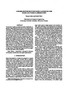
Fig. 3. (a) Size-128 Shepp-Logan phantom, (b) a star-shaped sampling domain in the frequency plane containing 30 radial lines, and reconstructions using (c) filtered back-projection, (d) NIHT, (e) GPSR-DB, and (f) approximate ExCoV schemes for the sampling pattern in (b). (a), (b), (c) PSNR = 18.9 dB (d) PSNR = 22.6 dB (e) PSNR = 29.3 dB (f) PSNR = 102.9 dB.

domain, as illustrated in Fig. 3(b); see also [25] and [41]. The sensing matrix is chosen as [2] (5.4) with sampling matrix and orthonormal sparsifying matrix constructed using selected rows of 2-D DFT matrix (yielding the corresponding 2-D DFT coefficients of the phantom image that are within the star-shaped domain) and inverse Haar wavelet transform matrix, respectively. Here, the are orthonormal, satisfying . The marows of trix is not explicitly stored but instead implemented via FFT and wavelet function handle in Matlab. The Haar wavelet coefficient vector of the image in Fig. 3(a) is sparse, with the . In the exnumber of nonzero elements equal to ample in Fig. 3(b), the samples are taken along 30 radial lines in the frequency plane, each containing 128 samples, which yields . Our performance metric is the peak signal-to-noise ratio (PSNR) of a wavelet coefficients estimate : dB

(5.5)

where and denote the smallest and largest elements of the image . We compare the following representative reconstruction methods that are feasible for large-scale data: • the standard filtered back-projection that corresponds to setting the unobserved DFT coefficients to zero and taking the inverse DFT, see [41]; • the debiased gradient-projection for sparse reconstruction method in [12, Sec. III.B] (labeled GPSR-DB) with conver-

N

Fig. 4. PSNR as a function of the normalized number of measurements =m, where the number of measurements changes by varying the number of radial lines in the star-shaped sampling domain.

and regularization parameter , both manually tuned to achieve good reconstruction performance; • the NIHT method in [25], terminating when the squared norm of the difference of the signal estimates of two con; secutive iterations is below • the approximate ExCoV method with averaging-window and initial value (4.2a), with signal estilength mation steps (4.15a) implemented using at most 300 conjugate-gradient steps. Fig. 3(c)–(f) present the reconstructed images by the above methods from the 30 radial lines given in Fig. 3(b). Approximate ExCoV manages to recover the original image almost perfectly, whereas the filtered back-projection method, NIHT and GPSR-DB have inferior reconstructions. gence threshold

QIU AND DOGANDZIC: VARIANCE-COMPONENT BASED SPARSE SIGNAL RECONSTRUCTION AND MODEL SELECTION

In Fig. 4, we vary the number of radial lines from 26 to 43, from 0.19 to 0.31. We observe the and, consequently, sharp performance transition exhibited by approximate ExCoV (corresponding to 29 radial lines) very close at to the theoretical minimum observation number, which is about 0.1 m. Approximate ExCoV twice the sparsity level meaachieves almost perfect reconstruction with surements. NIHT also exhibits a sharp phase transition, but at (corresponding to 33 radial lines), and GPSR-DB that does not have a sharp phase transition in the range of we considered; rather, the PSNR of GPSR-DB improves with . an approximately constant slope as we increase VI. CONCLUDING REMARKS We proposed a probabilistic model for sparse signal reconstruction and model selection. Our model generalizes the sparse Bayesian learning model, yielding a reduced parameter space. We then derived the GML function under the proposed probabilistic model that selects the most efficient signal representation making the best balancing between the accuracy of data fitting and compactness of the parameterization. We optiproved the equivalence of GML objective with the mization problem (1.1) and developed the ExCoV algorithm that searches for models with high GML objective function and provides corresponding empirical Bayesian signal estimates. ExCoV is automatic and does not require knowledge of the signal-sparsity or measurement-noise levels. We applied ExCoV to reconstruct one- and two-dimensional signals and compared it with the existing methods. Further research will include analyzing the convergence of ExCoV, applying the GML rule to automate iterative hard thresholding algorithms (along the lines of [27]), and constructing GML-based distributed compressed sensing schemes for sensor networks, see also [44] and references therein for relevant work on compressed network sensing. VII. APPENDIX We first present the EM step derivation (Appendix A and then prove Theorem 1 (Appendix B), since some results from Appendix A are used in Appendix B; the derivation of in (4.16) is given in Appendix C.

2945

APPENDIX A EM STEP DERIVATION To derive the EM iteration (4.11)–(4.12), we repeatedly apply the matrix inversion lemma [43, eq. (2.22), p. 424]:

(A.1a) and the following identity [43, p. 425]: (A.1b) where and are invertible square matrices. The prior pdf (2.4a) can be written as (A.2) where is the diagonal matrix with diagonal elements obtained by appropriately interleaving the variand . Hence, and in ance components (2.4b) are restrictions of the signal covariance matrix to the index sets and . In particular, is the matrix whose row and column indices beof elements of long to the set ; similarly, is the matrix of elements whose row and column indices belong to . of We treat the signal vector as the missing data; then, the complete-data log-likelihood function of the measurements and the missing data given follows from (2.1) and (A.2):

(A.3) where const denotes the terms that do not depend on and . From (A.3), the conditional pdf of given and is shown in (A.4) at the bottom of the page, yielding (A.5a) and (A.5b), shown at the bottom of the page, where was defined in (2.6b) and (A.5b) follows by applying (A.1a) and (A.1b). Then, (4.11a)

(A.4)

(A.5a) (A.5b)

2946

IEEE TRANSACTIONS ON SIGNAL PROCESSING, VOL. 58, NO. 6, JUNE 2010

and (4.11b) follow by setting and restricting the mean vector in (A.5b) to the sub-vectors according to the index sets and . Similarly, (4.11d) follows by restricting the rows and columns of the covariance matrix in (A.5b) to a square sub-matrix according to index set . Now,

5

(B.1c) (B.1d)

where was defined in (2.6b) and, since is a diag, onal matrix, . leads to Proof: Using (2.6b) and setting

where the second equality follows by restricting the rows and in (A.5b) to columns of the covariance matrix leads to (4.11e). Similarly, the index set . Setting

and (B.1a) follows by using the limiting form of the Moore– Penrose inverse [43, Th. 20.7.1]. Using (B.1a), we have

where the second term simplifies by using (A.1b) and (A.5b) [see (2.6b)]: and (B.1b) follows by noting that and has full column rank due to URP, see also [43, Th. 20.5.1]. Now, apply (A.1a): see the equation at the exists due bottom of the page, and note that and URP condition; (B.1c) then follows. Finally, to

and (4.11f) follows by setting . This concludes the derivation of the E step (4.11). The M step (4.12) easily follows by setting the derivatives of with respect to the variance components to zero. APPENDIX B PROOF OF THEOREM 1 We first prove a few useful lemmas. Lemma 1: Consider an index set with cardinality , defining distinct signal variance components. Assume that the URP condition (1) holds, distinct variance components are all positive, and the single variance for is zero, i.e., and , implying that is the set of indices corresponding to all positive signal variance components. Then, the following hold:

where the last term is finite when and URP condition (1) holds, and (B.1d) follows. Under the conditions of Lemma 1 and if , is unbounded as . Equation (B.1a)–(B.1c) show that multiplying by or leads to bounded limiting ex. When , behaves as pressions as as , see (B.1d); the smaller , grows to infinity. the quicker We now examine and the signal estimate [see (A.5b)]

(B.1a) (B.1b)

(B.2)

QIU AND DOGANDZIC: VARIANCE-COMPONENT BASED SPARSE SIGNAL RECONSTRUCTION AND MODEL SELECTION

for the cases where the index set does and does not includes -optimal support . the Lemma 2: As in Lemma 1, we assume that the URP condi, , and , implying tion (1) holds and that is the set of indices corresponding to all positive signal variance components. -optimal support ( ), a) If includes the then (B.3a) (B.3b) b) If

does not include the ) and

-optimal support , then

5 in

Proof: implies that the elements of are zero; consequently,

2947

Lemma 3: For any distinct-variance index set , define the index set of positive variance components in : (B.6a) with cardinality (B.6b) Assume that the URP and Fisher-information conditions (1) and (2) hold. , then (a) If

( if if

(B.3c) with indices

(b) If

, then

(B.4) and (B.3a)–(B.3b) follow by using (B.4), (B.1b), and (B.2). . Observe that, when We now show part (b) where ,

(B.7a)

if if Proof: Without loss of generality, let and block partition

(B.7b)

as (B.8)

We first show part (a), where (B.5) which follows by using (B.4) and partitioning into and . The first two terms in (B.5) are finite at , which easily follows by employing (B.1a) and (B.1b). Then, the equality in (B.3c) follows by using (B.1c). We now show that (B.3c) is positive by contradiction. The URP property of and the assumption that imply that the columns of are linearly independent. Since is a nonzero vector and columns of are linearly independent, is a nonzero vector. If (B.3c) is belongs to the column space zero, then of , which contradicts the fact that the columns of are linearly independent. Lemma 2 examines the behavior of and the signal estimate (B.2) as noise variance shrinks to zero. Clearly, is desirable and, in contrast, there is a severe penalty if . Under the assumptions of Lemma 2, [which is an important term in the log-likelihood function (2.6c)] is finite when includes all elements of , see (B.3a); in contrast, when misses any index from , grows hyperbolically with as , see (B.3c). Furthermore, if includes , (B.3b) holds regardless of the specific values of provided that they are positive; hence, the signal estimate will be -optimal even if the variance components are inaccurate. The next lemma studies the behavior of the Fisher information term of the GML function.

property of

implies that

and, therefore, . When , the URP and are finite matrices and (B.9)

and, consequently, Consider now the case where is unbounded as . Applying Lemma 1 to the index implies that multiplying by or leads to set bounded expressions; in particular, we obtain (B.10), shown at the bottom of the next page, where the limits in (B.10a)–(B.10e) are all finite; see also (3.4). and multiply We analyze the Fisher information matrix all terms that contain and are not guarded by . by rows and In particular, multiplying the last by , respectively, leads to (B.11), shown at columns of the bottom of the next page, and (B.7a) follows. and We now show part (b), where . When , the URP property of results in finite and, therefore, is also finite, leading to (B.12) When , we have (B.13). See equation (B.13) at the bottom of the next page, and (B.7b) follows by applying and arguments analogous to those in part Lemma 1 for (a).

2948

IEEE TRANSACTIONS ON SIGNAL PROCESSING, VOL. 58, NO. 6, JUNE 2010

From Lemma 3, we see that the Fisher information term of GML penalizes inclusion of zero variance components into index set . In the following lemma, we analyze ML . variance-component estimation for the full model and Lemma 4: Consider the full model with [see (2.3)], implying and the variempty , ance-component parameter vector equal to where . In this case, the log-likelihood function of the variance components is (2.6c) with . Assume that the URP and measurement number conditions (1) and (3) hold and consider that satisfy all

, is always finite; therefore, it can become inIf . Among all choices of finitely large only if for which is infinitely large, those defined by (B.14a) and (B.14b) “maximize” the likelihood in the sense that grows to infinity at the fastest rate as , quantified by (B.14c). Any choice of different from in (B.14a) cannot achieve this rate and, therefore, has a “smaller” likeli. hood than at satisfying (B.14a), i.e., Proof: Consider . Applying (B.1d) in Lemma 1 and (B.3a) in Lemma 2(a) for yields (B.14c) the index set

(B.14a) (B.14b) where

(B.14a)

states

that the support of is identical to the . Then, the log-likelihood at support as approaches proportionally to speed

-optimal grows , with

(B.14c)

(B.15) We now examine the model parameters different from in , is bounded and, therefore, the likelihood (B.14). If is always finite. Since we are interested in those for which the likelihood is infinitely large, we focus on the case

(B.10a) (B.10b)

5 (B.10c)

5 5 5

(B.10d) (B.10e)

(B.11)

(B.13)

QIU AND DOGANDZIC: VARIANCE-COMPONENT BASED SPARSE SIGNAL RECONSTRUCTION AND MODEL SELECTION

where and and partition the rest of the proof into three parts: with cardinality a) For

with

. Consider all variance-component estimates that satisfy

(B.16a) and , see (3.5). Applying (B.1d) and (B.3c) for (which satisfies the conditions of the index set Lemma 2(b)) yields

(B.19a) (B.19b)

we have

(B.16b) at . The penalty is and, consequently, -optimal support. high for missing the with cardinality that satisfies b) For (B.17a) and consider three cases: i) , ii) and , and iii) , i.e., is strictly larger than . For i), we apply the same approach as in a) above, and conclude that at . For ii), we observe and apply that (which satisfies the condi(B.1d) for the index set tions of Lemma 2(b)) to this upper bound, yielding

Then,

(B.20) , is always finite. Among all choices of If and for which is infinitely large, those and defined by (B.19a) and (B.19b) “maximize” the likelihood in the grows to infinity at the fastest rate as sense that , quantified by (B.20). Any choice of different from in (B.19a) cannot achieve this rate and, therefore, at . has a “smaller” likelihood than Proof: Corollary 5 follows from the fact that the model is nested within the full model . We refer to all defined by (B.19) as the ML estimates of under the scenario considered in Corollary 5. Proof of Theorem 1: The conditions of Lemma 3 and Corollary 5 are satisfied, since they are included in the the; by orem’s assumptions. Consider first the model Corollary 5, the ML variance-component estimates under this model are given in (B.19). Applying (B.20) and (B.7a) in yields Lemma 3 for

(B.21)

(B.17b) Therefore, that satisfy ii) have “smaller” likelihood (in the convergence speed sense defined in Lemma 4) than in (B.14a) at . For iii), arguments similar to those in (B.15) lead to (B.18) and, consequently, that satisfy iii) cannot match or out. perform at with cardinality , is bounded c) For is finite. and, therefore, With a slight abuse of terminology, we refer to all defined by (B.14) as the ML estimates of under the scenario considered in Lemma 4. Interestingly, the proof of Lemma 4 re, grows to infinity when veals that, as as well, but at a slower rate than that in (B.14c). In Corollary 5, we focus on the model where the index set is equal to the -optimal support and, consequently, . Corollary 5: Assume that the URP and measurement number conditions (1) and (3) hold and consider the model

2949

Hence, under the conditions of Theorem 1, is infinitely large. In the following, we show that, for any other model , in (3.1) is either finite or, if infinitely large, is smaller than that specthe rate of growth to infinity of ified by (B.21). Actually, it suffices to demonstrate that any with yields a “smaller” than , where has been defined in (B.19). , is bounded and, therefore, the resulting If is always finite. Consider the scenario where and and reand its cardinality in (B.6). call the definitions of is the set of indices corresponding to all posThen, . itive signal variance components, with cardinality Now, consider two cases: i) and ii) . For i), the URP condition (1) implies that is in (3.2) is finite. For ii), observe bounded and, therefore, that (B.22) apply (B.1d) in Lemma 1 for the index set that and in Lemma 1 have been replaced by

(meaning

2950

and 3(b), yielding

IEEE TRANSACTIONS ON SIGNAL PROCESSING, VOL. 58, NO. 6, JUNE 2010

, respectively), and use (B.7b) in Lemma

where the inequality follows from cannot exceed . fore, by (B.22), maximizes In summary, the model globally and uniquely. By (B.3b) in Lemma 2(a),

; therein (3.1) (B.27)

(B.23) where the last inequality follows from the assumption (2.2). goes to negative infinity as Therefore, by (B.22), . From i)–ii) above, we conclude that cannot exceed when and . We now focus our attention to the scenario where and . For any and any corresponding , consider four , ii’) and , cases: i’) and , and iv’) iii’) . For i’), is bounded and, therefore, is finite. For [see ii’), we have (3.5)] and, therefore,

where is the set of ML variance. component estimates in (B.19) for APPENDIX C DERIVATION OF Plugging (4.14a) and (4.14c) into (2.6b) and applying (A.1a) yields (C.1a) (C.1b) Approximating

by its diagonal elements (4.17) leads to (C.2a) (C.2b) (C.2c)

(C.2d)

(B.24) where we have applied (B.1d) in Lemma 1 and (B.3c) in Lemma , and used (B.7a) in Lemma 3(a); 2(b) for the index set goes to negative infinity as . Here, therefore, does not Lemma 2 (b) delivers the severe penalty since -optimal support . include the If iii’) holds, we apply (B.1d) in Lemma 1 and (B.3a) in and use (B.7a) Lemma 2(a) for the index set in Lemma 3(a), yielding

where (C.2e) (C.2f) for dependence of

; to simplify notation, we have omitted the and on . Furthermore,

(B.25) In this case, and the largest possible (B.25) , which is equivis attained if and only if ; then, (B.25) reduces to (B.21). For , alent to (B.25) is always smaller than the rate in (B.21), which is caused by inefficient modeling due to the zero variance components in the index set ; the penalty for this inefficiency is quantified by Lemma 3. For iv’), apply (B.1d) in Lemma 1 for the index set and use (B.7a) in Lemma 3(a), yielding

(C.2g)

(C.2h)

(C.2i)

(B.26)

(C.2j)

QIU AND DOGANDZIC: VARIANCE-COMPONENT BASED SPARSE SIGNAL RECONSTRUCTION AND MODEL SELECTION

We approximate (3.4b)–(3.4b) using (C.2h)–(C.2j) and use [see (4.13) and (4.14b)]: (C.3a)

(C.3b) (C.3c) yielding

(C.3d) and, using the formula for the determinant of a partitioned matrix [43, Th. 13.3.8]:

(C.4) Finally, the approximate GL formula (4.16) follows when we substitute (C.1), (C.2g), and (C.4) into (3.2). REFERENCES [1] I. F. Gorodnitsky and B. D. Rao, “Sparse signal reconstruction from limited data using FOCUSS: A re-weighted minimum norm algorithm,” IEEE Trans. Signal Process., vol. 45, no. 3, pp. 600–616, Mar. 1997. [2] E. Candès and J. Romberg, C. Bouman and E. Miller, Eds., “Signal recovery from random projections,” in Proc. SPIE-IS&T Electronic Imaging Computational Imaging III, San Jose, CA, Jan. 2005, vol. 5674, pp. 76–86. [3] E. J. Candès and T. Tao, “Decoding by linear programming,” IEEE Trans. Inf. Theory, vol. 51, pp. 4203–4215, Dec. 2005. [4] D. Malioutov, M. Çetin, and A. S. Willsky, “A sparse signal reconstruction perspective for source localization with sensor arrays,” IEEE Trans. Signal Process., vol. 53, no. 8, pp. 3010–3022, Aug. 2005. [5] E. J. Candès, J. Romberg, and T. Tao, “Stable signal recovery from incomplete and inaccurate information,” Commun. Pure Appl. Math., vol. 59, pp. 1207–1233, Aug. 2006. [6] IEEE Signal Process. Mag. (Special Issue on Sensing, Sampling, and Compression), Mar. 2008. [7] A. M. Bruckstein, D. L. Donoho, and M. Elad, “From sparse solutions of systems of equations to sparse modeling of signals and images,” in SIAM Rev., Mar. 2009, vol. 51, pp. 34–81. [8] B. K. Natarajan, “Sparse approximate solutions to linear systems,” SIAM J. Comput., vol. 24, pp. 227–234, Apr. 1995. [9] S. Chen, D. Donoho, and M. Saunders, “Atomic decomposition by basis pursuit,” SIAM J. Sci. Comput., vol. 20, no. 1, pp. 33–61, 1998. [10] E. Candès and T. Tao, “The Dantzig selector: Statistical estimation when p is much larger than n,” Ann. Stat., vol. 35, pp. 2313–2351, Dec. 2007. [11] R. Tibshirani, “Regression shrinkage and selection via the lasso,” J. R. Stat. Soc., Ser. B, vol. 58, pp. 267–288, 1996. [12] M. A. T. Figueiredo, R. D. Nowak, and S. J. Wright, “Gradient projection for sparse reconstruction: Application to compressed sensing and other inverse problems,” IEEE J. Sel. Topics Signal Process., vol. 1, no. 4, pp. 586–597, Dec. 2007. [13] S. Mallat and Z. Zhang, “Matching pursuits with time-frequency dictionaries,” IEEE Trans. Signal Process., vol. 41, no. 12, pp. 3397–3415, 1993. [14] J. A. Tropp and A. C. Gilbert, “Signal recovery from random measurements via orthogonal matching pursuit,” IEEE Trans. Inf. Theory, vol. 53, pp. 4655–4666, Dec. 2007.

2951

[15] D. L. Donoho, Y. Tsaig, I. Drori, and J.-L. Starck, Sparse solution of underdetermined linear equations by Stagewise Orthogonal Matching Pursuit (StOMP),” http://www-stat.standford.edu/~donoho/reports/ html. [16] D. Needell and J. A. Tropp, “CoSaMP: Iterative signal recovery from incomplete and inaccurate samples,” Appl. Comput. Harmon. Anal., vol. 26, pp. 301–321, May 2009. [17] W. Dai and O. Milenkovic, “Subspace pursuit for compressive sensing signal reconstruction,” IEEE Trans. Inf. Theory, vol. 55, pp. 2230–2249, May 2009. [18] D. P. Wipf and B. D. Rao, “Sparse Bayesian learning for basis selection,” IEEE Trans. Signal Process., vol. 52, pp. 2153–2164, Aug. 2004. [19] D. P. Wipf and B. D. Rao, “Comparing the effects of different weight distributions on finding sparse representations,” in Adv. Neural In. Process. Syst., Y. Weiss, B. Schölkopf, and J. Platt, Eds. Cambridge, MA: MIT Press, 2006, vol. 18, pp. 1521–1528. [20] S. Ji, Y. Xue, and L. Carin, “Bayesian compressive sensing,” IEEE Trans. Signal Process., vol. 56, no. 6, pp. 2346–2356, Jun. 2008. [21] M. E. Tipping, “Sparse Bayesian learning and the relevance vector machine,” J. Mach. Learn. Res., vol. 1, pp. 211–244, 2001. [22] K. K. Herrity, A. C. Gilbert, and J. A. Tropp, “Sparse approximation via iterative thresholding,” in Proc. Int. Conf. Acoust., Speech, Signal Processing, Toulouse, France, May 2006, pp. 624–627. [23] T. Blumensath and M. E. Davies, “Iterative thresholding for sparse approximations,” J. Fourier Anal. Appl., vol. 14, pp. 629–654, Dec. 2008. [24] T. Blumensath and M. E. Davies, “Iterative hard thresholding for compressed sensing,” Appl. Comput. Harmon. Anal., vol. 27, pp. 265–274, Nov. 2009. [25] T. Blumensath and M. E. Davies, “Normalized iterative hard thresholding: Guaranteed stability and performance,” IEEE J. Sel. Topics Signal Process., vol. 4, no. 2, pp. 298–309, 2010. [26] A. Maleki and D. L. Donoho, “Optimally tuned iterative thresholding algorithms for compressed sensing,” IEEE J. Sel. Topics Signal Process., vol. 4, no. 2, pp. 330–341, 2010. [27] A. Dogandzic and K. Qiu, “Automatic hard thresholding for sparse signal reconstruction from NDE measurements,” in Rev. Progress Quantitat. Nondestruct. Eval., AIP Conf. Proc., D. O. Thompson and D. Chimenti, Eds., Melville, NY, 2010, vol. 29, pp. 806–813. [28] K. Qiu and A. Dogandzic, “Double overrelaxation thresholding methods for sparse signal reconstruction,” presented at the 44th Annu. Conf. Inf. Sci. Syst., Princeton, NJ, Mar. 2010. [29] B. D. Rao and K. Kreutz-Delgado, “An affine scaling methodology for best basis selection,” IEEE Trans. Signal Process., vol. 47, no. 1, pp. 187–200, Jan. 1999. [30] E. J. Candès, M. B. Wakin, and S. P. Boyd, “Estimating sparsity by reweighted ` minimization,” J. Fourier Anal. Appl., vol. 14, pp. 877–905, Dec. 2008. [31] R. Chartrand and W. Yin, “Iteratively reweighted algorithms for compressive sensing,” in Proc. Int. Conf. Acoust., Speech, Signal Process., Las Vegas, NV, Apr. 2008, pp. 3869–3872. [32] S. M. Kay, Fundamentals of Statistical Signal Processing: Detection Theory. Englewood Cliffs, NJ: Prentice-Hall, 1998. [33] M. H. Hansen and B. Yu, “Model selection and the principle of minimum description length,” J. Amer. Stat. Assoc., vol. 96, pp. 746–774, Jun. 2001. [34] J. Rissanen, Information and Complexity in Statistical Modeling. New York: Springer-Verlag, 2007. [35] A. Dogandzic and K. Qiu, “ExCoV: Expansion-compression variance-component based sparse-signal reconstruction from noisy measurements,” in Proc. 43rd Annu. Conf. Inform. Sci. Syst., Baltimore, MD, Mar. 2009, pp. 186–191. [36] S. M. Kay, Fundamentals of Statistical Signal Processing: Estimation Theory. Englewood Cliffs, NJ: Prentice-Hall, 1993. [37] D. L. Donoho and J. Tanner, “Counting faces of randomly projected polytopes when the projection radically lowers dimension,” J. Amer. Math. Soc., vol. 22, pp. 1–53, Jan. 2009. [38] A. P. Dempster, N. M. Laird, and D. B. Rubin, “Maximum likelihood from incomplete data via the EM algorithm,” J. R. Stat. Soc., Ser. B, vol. 39, pp. 1–38, Jul. 1977. [39] G. J. McLachlan and T. Krishnan, The EM Algorithm and Extensions, 2nd ed. New York: Wiley, 2008. [40] Å. Björck, Numerical Methods for Least Squares Problems. Philadelphia, PA: SIAM, 1996. [41] E. J. Candès, J. Romberg, and T. Tao, “Robust uncertainty principles: Exact signal reconstruction from highly incomplete frequency information,” IEEE Trans. Inf. Theory, vol. 52, pp. 489–509, Feb. 2006. [42] S.-J. Kim, K. Koh, M. Lustig, S. Boyd, and D. Gorinevsky, “An interior-point method for large-scale ` -regularized least squares,” IEEE J. Sel. Topics Signal Process., vol. 1, no. 4, pp. 606–617, Dec. 2007.

2952

IEEE TRANSACTIONS ON SIGNAL PROCESSING, VOL. 58, NO. 6, JUNE 2010

[43] D. A. Harville, Matrix Algebra From a Statistician’s Perspective. New York: Springer-Verlag, 1997. [44] C. Luo, F. Wu, J. Sun, and C. W. Chen, “Compressive data gathering for large-scale wireless sensor networks,” in Proc. Int. Conf. Mobile Comput. Networking (MobiCom), Beijing, China, Sep. 2009, pp. 145–156.

Kun Qiu (S’07) was born in Shanghai, China. He received the B.S. degree in electrical engineering from Fudan University, Shanghai, China, in 2006. He is working towards the Ph.D. degree in the Department of Electrical and Computer Engineering, Iowa State University, Ames. His research interests are in statistical signal processing and its applications to sparse signal reconstruction and compressive sampling.

Aleksandar Dogandzic (S’96–M’01–SM’06) received the Dipl.Ing. degree (summa cum laude) in electrical engineering from the University of Belgrade, Yugoslavia, in 1995 and the M.S. and Ph.D. degrees in electrical engineering and computer science from the University of Illinois at Chicago (UIC) in 1997 and 2001, respectively. In August 2001, he joined the Department of Electrical and Computer Engineering, Iowa State University (ISU), Ames, where he is currently an Associate Professor. His research interests are in statistical signal processing theory and applications. Dr. Dogandzic received the 2003 Young Author Best Paper Award and 2004 Signal Processing Magazine Best Paper Award, both by the IEEE Signal Processing Society. In 2006, he received the CAREER Award by the National Science Foundation. At ISU, he was awarded the 2006–2007 Litton Industries Assistant Professorship in Electrical and Computer Engineering. Dr. Dogandzic serves as an Associate Editor for the IEEE TRANSACTIONS ON SIGNAL PROCESSING and the IEEE SIGNAL PROCESSING LETTERS.