distribution is a good starting point in order to deal with class imbalance. 1 Introduction ... choice as AUC values near the balanced distribution are often the best.
A Study with Class Imbalance and Random Sampling for a Decision Tree Learning System Ronaldo C. Prati, Gustavo E. A. P. A Batista, and Maria Carolina Monard
Abstract Sampling methods are a direct approach to tackle the problem of class imbalance. These methods sample a data set in order to alter the class distributions. Usually these methods are applied to obtain a more balanced distribution. An open-ended question about sampling methods is which distribution can provide the best results, if any. In this work we develop a broad empirical study aiming to provide more insights into this question. Our results suggest that altering the class distribution can improve the classification performance of classifiers considering AUC as a performance metric. Furthermore, as a general recommendation, random over-sampling to balance distribution is a good starting point in order to deal with class imbalance.
1 Introduction A key point for the success of Machine Learning – ML – application in Data Mining is related to understanding and overcoming some practical issues that have not been previously considered when learning algorithms were initially proposed. One of these issues that has come into light in supervised learning is related to class imbalance, where some classes are represented by a large number of examples while the others are represented by only a few. Numerous studies report a poor performance of the induced models in domains where class imbalance is present[2, 10]. Sampling methods are a direct approach to tackle the problem of class imbalance. These methods sample a data set in order to alter the class distributions. Usually these methods are applied in order to obtain a more balUniversity of S˜ ao Paulo P. O. Box 668, ZIP Code 13560-970 S˜ ao Carlos (SP), Brazil e-mail: {prati,gbatista,mcmonard}@icmc.usp.br
Ronaldo C. Prati, Gustavo E. A. P. A Batista, and Maria Carolina Monard
anced distribution. The two most well-known sampling methods to deal with the problem of class imbalance are random over-sampling and random undersampling. These methods replicate (eliminate) examples of the minority (majority) class in order to obtain a more balanced distribution. An open-ended question considering sampling methods is which distribution can provide the best results, if any. In this work we develop a broad empirical study aiming to provide more insights into this question. To this end, random under-sampling and random over-sampling methods were used to change the class distribution of fourteen UCI [1] data sets. The data sets are under and over-sampled to reach thirteen different fixed class distributions and used as input to a decision tree learning algorithm (C4.5) to induce a model. Our results suggest that altering the class distribution can improve the classification performance of classifiers considering AUC as the performance metric. Furthermore, as a general recommendation given the results obtained, random over-sampling can be considered a good starting point to deal with class imbalance. This method is straightforward to implement and considerably fast if compared with more sophisticated (heuristic) sampling methods. Oversampling attempting to reach the balanced distribution is also a good first choice as AUC values near the balanced distribution are often the best. This work is organized as follows: Section 2 presents some notes on ROC analysis, and its importance in evaluating the performance of classifiers in imbalanced domains. Section 3 discusses our methodology and the experimental results obtained. Finally, Section 4 presents some concluding remarks as well as outlines some future research.
2 ROC analysis From hereafter, we constrain our analysis to two-class problems, where the minority class will be called positive and the majority class negative. A straightforward connection between class imbalance and error rate might be traced by observing that it is easier to achieve a low overall error rate by simply predicting the majority class. For instance, it is straightforward to create a classifier having an error rate of 1% in a domain where the majority class proportion corresponds to 99% of the instances, by simply forecasting every new example as belonging to the majority class. In scenarios where the target class priors and/or misclassification costs are unknown or are likely to change, the use of error rate as a basic performance measure may lead to misleading conclusions. This is due to the fact that the error rate strongly depends on class distribution and misclassification costs. Furthermore, the use of the error rate in such conditions does not allow the direct comparison/evaluation of how learning algorithms would perform in different scenarios. In a nutshell, two fundamental aspects of performance,
A Study with Class Imbalance and Random Sampling for a DT
namely discrimination capacity and decision tendencies1 , are confused when error rate is used as a basic performance measure. Often, we are primarily interested in the discrimination aspect. In this case we want to leave out the decision aspect such that it does not mislead the evaluation of classifiers. Receiver Operating Characteristic (ROC) analysis [8] provides such a way of assessing a classifier performance independently of the criterion adopted for making a particular decision on how to trade-off true/false positives as well as the bias used by learning algorithms toward one particular decision or another. Thus, ROC based methods provide a fundamental tool for analyzing and assessing classifiers performance in imprecise environments. The basic idea is to decouple relative error rate (percentage of false positives or false positive rate – F Prate ) from hit rate (percentage of true positives or true positive rate – T Prate ) by using each of them as axis in a bi-dimensional space. Thus, in ROC analysis a classifier is represented by a pair of values instead of a single error rate value. Furthermore, spreading the classifier criterion over all possible trades off of hits and errors, a curve that works as an index that reflects the subjective probabilities and utilities that determine all possible criteria is obtained. For instance, considering a classifier that provides probabilities of an example belonging to each class, such as the Naive Bayes classifier, we can use these probabilities as a threshold parameter biasing the final class selection. Then, for each threshold, we plot the percentage of hits against the percentage of errors. The result is a bowed curve, rising from the lower left corner (0,0), where both percentages are zero, to the upper right corner (1,1), where both percentages are 100%. The more sharply the curve bends, the greater the ability of coping with different class proportions and misclassification costs, since the number of hits relative to the number of false alarms is higher. By doing so, it is possible to consider what might happen if a particular score is selected as a classification threshold, allowing to select the most suitable threshold given a specific situation. In situations where neither the target cost distribution nor the class distribution are known, an alternative metric to compare models through ROC analysis is the area under the ROC curve (AUC). The AUC represents the probability that a randomly chosen positive example will be rated higher than a negative one [12], and in this sense it is equivalent to the Wilcoxon test of ranks. However, it should be kept in mind that given a specific target condition, the classifier with the maximum AUC may not be the classifier with the lowest error rate. 1
Discrimination capacity can be defined as how well the system is able to discriminate between positive and negative examples. Decision tendencies can be understood as how well the system is able to manage the trade-off between true and false positives given different misclassification costs and class distribution scenarios.
Ronaldo C. Prati, Gustavo E. A. P. A Batista, and Maria Carolina Monard
3 Experiments The experiments involved the application of two sampling methods to fifteen UCI [1] data sets. We start describing the sampling methods and the methodology used in the experiments, followed by an analysis of the results obtained. The two sampling methods used in the experiments with the objective of altering the class distribution of training data are: Random under-sampling: a method that reduces the number of examples of one of the classes through the random elimination of examples of this class. Random over-sampling: a method that increases the number of examples of one of the classes through the random replication of examples of this class. Usually, random under-sampling and random over-sampling are used to approximate the prior probabilities of each class. Therefore, random undersampling is usually applied to the majority (negative) class while random over-sampling is usually applied to the minority (positive) class. Several authors agree that the major drawback of random under-sampling is that this method can discard potentially useful data that could be important to the induction process. On the other hand, random over-sampling supposedly increases the likelihood of occurring overfitting, since it makes exact copies of the minority class examples. For instance, a symbolic classifier might construct rules that are apparently accurate although actually cover one replicated example. For experimental analysis, we selected fourteen data sets from UCI [1] having different degrees of imbalance. Table 1 summarizes the data sets used in this study. For each data set, it shows the number of examples (#Examples), number of attributes (#Attributes), together with the number of quantitative and qualitative attributes in brackets, class labels and class distribution. For data sets having more than two classes, we chose the class with fewer examples as the positive class, and collapsed the remainder as the negative class. Our implementation of random over-sampling and random under-sampling methods have a parameter that allows the user to set up the desired class distribution that should be reached after the application of these methods. We over and under-sampled all data sets until the following positive class distributions were reached: 5%, 7.5%, 10%, 20%, 30%, 40%, 50%, 60%, 70%, 80%, 90%, 92.5% and 95%. Distributions greater than 50% mean that the application of the over or under-sampling methods made the positive class more frequent than the negative class. Moreover, in order to reach distributions smaller (more imbalanced) than the original ones, we over-sampled the negative class or under-sampled the positive class, depending on which method was being applied.
A Study with Class Imbalance and Random Sampling for a DT Table 1 Data sets summary descriptions. # 1 2 3 4 5 6 7 8 9 10 11 12 13 14
Data set #Attributes Class #Examples Name (min., maj.) (positive,negative) sonar 208 61 (61,0) (m, r) heart 270 14 (14,0) (2, 1) bupa 345 7 (7,0) (1, 2) ionosphere 351 34 (34,0) (bad, good) breast 683 10 (10,0) (malignant, benign) pima 768 8 (8,0) (1, 0) tic-tac-toe 958 10 (0,10) (positive, negative) german 1000 20 (7,13) (bad, good) haberman 306 3 (3,0) (die, survive) vehicle 846 18 (18,0) (van, remainder) new-thyroid 215 5 (5,0) (hypo, remainder) ecoli 336 7 (7,0) (imu, remainder) flag 194 28 (10,18) (white, remainder) glass 214 9 (9,0) (ve-win-float-proc, remainder)
Class proportion (46.6%, 53.5%) (44.4%, 55.6%) (42.0%, 58.0%) (35.9%, 64.1%) (35.0%, 65.0%) (34.8%, 65.2%) (34.7%, 65.3%) (30.0%, 70.0%) (26.5%, 73.5%) (23.5%, 76.5%) (16.3%, 83.7%) (10.4%, 89.6%) (8.8%, 91.2%) (7.9%, 92.1%)
It is important to note that, as under and over-sampling are applied, the number of training examples will vary. In particular, the number of training examples of under-sampled data sets might be significantly reduced. This shortcoming is one of the most frequent criticisms regarding under-sampling as this method might discard important information. It should be observed that our experimental setup is significantly different from [14], where Weiss & Provost consider a scenario in which data are expensive to acquire, and they analyze the effect of class distribution. Their experimental setup uses random under-sampling, however training set sizes are constant for all class distributions. In our experiments release 8 of the C4.5 [13] symbolic learning algorithm was used to induce decision trees. The trees were induced with default parameter settings. m-estimation [4] was used to improve the leaf probability estimates to produce ROC curves. We adjusted the m parameter so that bm = 10 as suggested in [6], where b is the prior probability of the positive class. We also use the AUC as the main method to assess our experiments. Table 2 presents the AUC values obtained by the trees induced by C4.5 with random under and over-sampled data sets. The first column in Table 2 specifies the number of the data set (according to Table 1) and the next two columns specify the natural proportion of positive examples followed by the AUC values assessed using this distribution. The next columns present the AUC values for the thirteen fixed class distributions. Each line has been split into two, each one presenting the results obtained with random over and under-sampled data sets, as indicated in the fourth column. All AUC values in Table 2 were obtained using 10-fold stratified cross-validation, and the values between brackets refer to the standard deviations. The highest AUC values for each data set/method are shaded. The last column (p-value) shows the p-value of the statistical test comparing the shaded results with the natural distribution. The statistical procedure used to carry out the tests is the Student paired t-test, with the null hypothsis (H0 ) that
Ronaldo C. Prati, Gustavo E. A. P. A Batista, and Maria Carolina Monard
Table 2 AUC results for random under (Ud) and over (Ov) sampling methods for several positive class distributions.
Ov Ud Ov Ud Ov Ud Ov Ud Ov Ud Ov Ud Ov Ud Ov Ud Ov Ud Ov Ud Ov Ud Ov Ud Ov Ud Ov Ud
Original Proportion of positive examples # Smp p-value Prp AUC 95% 92.5% 90% 80% 70% 60% 50% 40% 30% 20% 10% 7.5% 5% 68.4(9.4) 68.5(10.0)73.8(12.3) 77.5(11.3) 71.5(12.5)80.6(10.8) 79.1(12.6) 77.7(7.3) 73.8(12.1)70.9(13.1) 73.5(12.6) 71.5(8.4) 74.3(12.5) 0.37 1 46.6 79.0(11.0) 53.3(10.6)55.0(12.3) 56.0(8.4) 75.7(17.3) 77.5(15.6) 72.7(17.9) 78.4(10.6) 78.8(14.9) 70.6(12.4) 65.9(9.9) 66.8(12.2) 65.5(11.7) 62.3(10.0) 0.49 82.2(14.3)84.5(14.3)87.3(10.1)88.1(10.3) 87.2(9.4) 84.1(10.0) 84.2(9.0) 85.6(11.0) 87.6(9.1) 84.7(10.3) 86.1(12.4) 87.6(9.4) 87.3(8.6) 0.29 2 44.4 85.5(10.4) 53.1(9.9) 62.5(16.3)74.0(20.7) 79.5(11.9) 84.9(9.8) 86.8(8.8) 87.0(6.9) 88.4(10.6) 88.8(8.2) 82.6(11.4) 70.8(8.5) 65.7(10.0) 59.1(9.2) 0.22 63.1(6.8) 65.6(6.0) 65.1(9.6) 65.4(8.6) 61.6(6.6) 64.1(9.5) 68.0(9.6) 64.5(7.4) 65.1(6.5) 66.3(4.6) 67.1(4.5) 65.0(8.3) 66.2(7.7) 0.23 3 42.0 65.2(6.6) 50.0(0.0) 49.6(1.5) 52.7(7.1) 57.1(7.2) 61.3(10.8) 61.8(9.1) 64.0(6.6) 62.9(6.2) 61.1(7.4) 55.4(8.6) 57.3(9.2) 53.2(7.9) 50.8(2.5) 0.22 89.4(6.6) 89.7(5.8) 91.8(4.6) 92.2(4.9) 91.9(4.3) 92.7(4.7) 92.8(6.4) 92.7(3.7) 91.3(5.1) 92.9(4.1) 90.2(5.3) 90.9(5.8) 89.4(6.6) 0.24 4 35.9 91.4(5.0) 66.0(10.6) 75.8(5.9) 79.6(6.0) 88.2(6.2) 89.6(5.8) 92.0(5.2) 90.2(6.0) 90.4(4.4) 89.1(4.2) 89.2(5.2) 85.8(5.9) 83.6(6.7) 82.1(9.3) 0.40 97.1(2.7) 97.2(2.7) 97.1(2.6) 97.1(2.5) 96.9(2.6) 97.4(2.0) 97.3(2.2) 96.5(2.5) 97.3(1.9) 96.5(3.6) 96.5(2.5) 96.9(3.5) 96.8(3.6) 0.117 5 35.0 95.7(3.9) 89.8(4.3) 91.7(5.0) 92.5(3.8) 93.2(2.9) 94.9(2.7) 95.8(2.1) 95.4(2.7) 96.3(3.4) 96.3(2.2) 96.1(2.9) 95.4(3.5) 93.8(5.3) 91.4(6.3) 0.34 76.7(7.0) 77.0(6.7) 77.3(7.5) 78.2(7.3) 77.3(8.2) 76.9(4.5) 79.1(5.3) 79.6(6.8) 75.7(6.9) 78.6(5.3) 78.3(7.2) 78.9(6.9) 79.4(5.2) 0.41 6 34.8 79.0(5.1) 60.8(10.0) 69.1(6.0) 69.2(5.9) 73.6(8.0) 77.9(5.2) 77.1(4.9) 80.2(6.1) 78.7(6.1) 78.8(6.2) 72.6(7.1) 63.7(10.5) 61.1(11.6) 57.7(9.0) 0.32 93.1(2.7) 93.0(3.4) 92.7(3.4) 92.3(3.6) 92.1(4.0) 93.1(3.1) 91.5(3.7) 90.8(4.5) 88.8(2.4) 90.1(3.3) 89.2(3.8) 87.3(5.9) 86.6(5.8) 0.06 7 34.7 91.0(3.0) 50.0(0.0) 51.7(5.2) 53.4(6.0) 76.0(6.3) 78.3(5.8) 83.8(5.6) 87.8(5.4) 87.8(4.4) 84.9(4.5) 75.7(7.9) 69.6(9.4) 59.5(10.9) 52.4(5.0) 0.04 69.9(6.1) 70.9(5.8) 69.1(4.8) 72.2(5.0) 70.9(4.0) 71.8(6.4) 72.5(5.9) 71.3(5.9) 72.6(4.0) 72.1(4.1) 73.2(4.3) 71.9(4.0) 72.4(4.5) 0.46 8 30.0 72.4(3.9) 50.0(0.0) 51.1(3.4) 50.0(0.0) 65.4(9.8) 70.4(7.9) 71.9(7.5) 70.4(5.9) 72.7(6.1) 72.8(4.0) 69.8(7.9) 50.0(0.0) 50.0(0.0) 50.0(0.0) 0.42 60.5(7.2) 62.6(9.2) 62.9(7.8) 59.7(9.9) 62.5(10.0) 63.8(10.3) 64.1(12.2) 61.3(10.6) 64.3(14.7) 51.2(5.3) 54.9(13.2) 52.9(7.4) 52.6(8.7) 0.04 9 26.5 54.1(7.9) 50.0(0.0) 50.4(6.0) 52.1(6.7) 49.7(1.9) 54.9(7.8) 59.7(10.2) 61.7(11.4) 63.2(13.2) 61.0(14.4) 50.0(3.9) 50.4(1.4) 50.4(1.4) 49.7(1.0) 0.04 97.7(1.8) 97.9(1.4) 97.9(1.1) 98.2(1.1) 98.1(2.1) 97.9(2.1) 97.8(2.0) 97.7(1.8) 97.8(1.5) 97.9(2.1) 97.9(2.2) 97.9(1.8) 97.7(2.3) 0.45 1023.5 98.1(2.0) 75.6(7.0) 84.7(9.0) 87.5(7.8) 94.6(3.8) 95.3(2.8) 96.5(2.9) 97.3(2.5) 97.3(2.4) 97.5(1.8) 97.8(1.9) 97.5(2.3) 96.5(2.6) 94.0(3.3) 0.37 91.2(18.9)91.2(18.9)91.2(18.9) 91.2(18.9) 91.2(18.9) 90.6(18.7) 90.6(18.7) 90.6(18.7) 90.3(18.5)84.3(21.1) 87.9(18.2) 85.9(19.0) 92.6(10.7) 0.31 1116.3 89.0(18.8) 55.3(14.2)89.2(12.2)88.2(10.1) 89.5(7.4) 85.0(16.5) 85.8(16.9) 87.7(17.8) 89.4(18.3) 87.5(18.1)86.0(19.0) 92.6(12.7) 92.8(14.5) 86.4(18.3) 0.31 94.9(5.5) 94.6(5.8) 94.3(6.8) 94.7(7.0) 94.3(7.2) 94.2(7.2) 93.1(6.7) 95.1(6.0) 95.2(6.2) 94.6(5.0) 92.7(8.3) 89.6(13.1) 93.3(9.0) 0.20 1210.4 92.5(8.1) 69.8(13.9)70.8(13.1)72.9(10.1) 84.2(7.0) 85.8(5.6) 89.3(6.7) 93.1(4.2) 94.0(3.9) 93.0(2.9) 85.4(14.3) 94.3(4.4) 83.5(15.5) 80.3(20.0) 0.30 66.2(22.8)67.8(24.2)67.0(23.3)69.3(25.4) 66.5(26.5) 66.7(27.1) 63.4(17.5) 63.1(21.5) 55.8(22.8)60.0(22.9) 49.2(1.9) 50.0(0.0) 50.0(0.0) 0.01 13 8.8 50.0(0.0) 50.0(0.0) 50.0(0.0) 50.8(2.6) 50.9(8.5) 60.5(6.6) 64.7(21.6) 59.3(29.7) 67.5(24.6) 64.6(28.1)49.9(23.7) 50.0(0.0) 50.0(0.0) 50.0(0.0) 0.02 85.4(14.7)81.8(15.6)82.2(15.6) 82.6(16.5) 82.9(15.3) 85.4(14.9) 85.6(15.5) 86.1(14.3) 85.0(17.0)83.4(18.0) 84.1(17.6) 82.9(19.3) 85.8(15.5) 0.31 50.0(0.0) 50.0(0.0) 56.5(6.5) 57.6(6.3) 63.9(19.3) 65.3(23.0) 67.1(16.8) 74.4(22.1) 69.3(22.0)79.0(19.8)83.4(18.0) 62.9(21.3) 51.7(5.3) 0.45 14 7.9 82.4(19.2)
A Study with Class Imbalance and Random Sampling for a DT
both means are the same. The smaller the p-value, the more evidence we have against H0 . A p-value lower than 0.05 indicates a 95% degree of confidence of rejecting H0 . Even though there are only a few differences at that significance level, some tendencies can be observed from these results. A first observation from Table 2 is that random over-sampling performs better than random under-sampling. Out of 15 data sets used in this study, in only 3 of them (heart(2) 2 , pima(6) and new-thyroid(11) ) under-sampling performed slightly better than over-sampling. The reason is two-fold: oversampling does not discard any cases and consequently it might not end up with a restricted set of examples which is unrepresentative of the underlying concept; and over-sampling increases the number of examples of the minority class, directly dealing with the problem of learning from the rare cases of this class. Another observation is that changing the class distribution seems to be worth the effort. For random over-sampling, the best results obtained for each data set are higher than the performance obtained with the original class distribution. For random under-sampling, results seem to be less promising as for 5 (sonar(1) , bupa(3) , tic-tac-toe(7) and vehicle(10) ) of the 15 data sets, random under-sampling was not able to improve the performance obtained with the original class distribution. As mentioned before, the best results obtained by over and under-sampling are shaded in gray. Most of these results are related to the most balanced class distributions, having a slight tendency to the left where, proportions are biased for the positive class. Three of the most balanced distributions, i.e., 40%, 50% and 60% of positive class prevalence, concentrate exactly 7 (50%) of the best results obtained by random over-sampling. If we restrict the analysis to the balanced distribution, random over-sampling provided performance results slightly better than the balanced distribution in 13 out of the 15 data sets. Specifically for data sets haberman(9) and flag(13) which have less than 30% of positive examples and poor classification performance, and consequently, seem to suffer from the class imbalance problem, random over-sampling to the balanced distribution was able to improve the performance in two of them (haberman(9) and flag(13) ) with a statistical confidence of 95%3 . It is important to note that the data sets german(8) , vehicle(10) , newthyroid(11) , ecoli(12) and glass(14) also have 30% or less positive class prevalence and do not seem to suffer from the class imbalance problem. For these data sets, balancing the class distribution did not improve the performance significantly. In addition, these data sets seem to confirm the hypothesis that the class imbalance does not hinder the performance of classifiers per se. 2
From hereafter, we use a subscript number after a data set name in order to facilitate references to Table 2. 3 For data set flag (13) , the Student t-test p-value between the balanced distribution and the natural distribution is 2.42. It is not shown in Table 2 since the balanced distribution did not provide the best result for all considered distributions.
Ronaldo C. Prati, Gustavo E. A. P. A Batista, and Maria Carolina Monard
Class imbalance must be associated with other data characteristics such as the presence of within-class imbalance and small disjuncts [9] and data overlapping [11] in order to cause a loss in performance. As a general recommendation given the results obtained in the experiments, random over-sampling seems to be a good starting point in order to deal with class imbalance. This method is straightforward to implement and considerably fast if compared with more sophisticated (heuristical) sampling methods. Over-sampling for the balanced distribution seems also to be a good first choice as AUC values near the balanced distribution are often the best. As mentioned early, another point that is often cited in the literature is that over-sampling may lead to overfitting, due to the fact that random over-sampling makes exact copies of minority class examples. As results related to random over-sampling and overfitting are often reported using error rates as the basic performance measure, we believe that the conclusions reported might be due to the confusion of the classification criteria and the discrimination ability natural to the error rate measure. As a matter of fact, over-sampled data sets might produce classifiers with higher error rates than the ones induced from the original distribution. Since it is not possible to determine the appropriate configuration without knowing in advance the target distribution characteristics, it is not possible to confirm that over-sampling leads to overfitting. In fact, the apparent overfitting caused by over-sampling might be a shift into the classification threshold in the ROC curve. Although for most of the sampled data sets it was not possible to identify significantly differences from the original distribution, this does not mean that the different sampling strategies or different proportions perform equally well, and that there is not any advantage in using one or another in a given situation. As stated earlier, this is due to the fact that the classifier with higher AUC values does not necessarily lead to the best classifier in the whole ROC space. The main advantage of using different sampling strategies relies on the fact that they could improve on different regions of the ROC space. In this sense, the sampling strategies and proportions could boost some rules that could be overwhelmed by imbalanced class distributions. For instance, consider the ROC curves shown in Figure 1. This figure presents ROC graphs (averaged over the 10 folds using the vertical average method described in [8]) for the pima(6) data set. Furthermore, we have selected two curves which perform well in different parts of the ROC space. The selected curves are those generated from random under-sampled data sets with class distribution of 70% positive examples and random over-sampled data sets with 20% positive examples. Figure 1 shows that random undersampling with 70% positive examples performs better in the range 0-50% of false positives, approximately. On the other hand, random over-sampled data sets with 20% positive examples outperforms random under-sampled data sets with 70% in the remainder of the ROC space. In other words, different sampling strategies and different class distribution may lead to improvements in different regions of the ROC space.
A Study with Class Imbalance and Random Sampling for a DT
4 Concluding remarks As long as learning algorithms use heuristics designed foroverall error rate minimization, it is natural to believe that these algorithms would be biased to perform better at classifying majority class examples than minority class ones, as the former is weighed more heavily when assessing the error rate. However, it is possible to use learning algorithms that use basic heuristics insensitive to class distribution. One of these algorithms (a decision tree using DKM splitting criterion) is shown to be competitive to overall error minimization algorithms in various domains [5]. Furthermore, for some domains standard learning algorithms are able to perform quite well no matter how skewed the class distribution is, even if the applied algorithms are (at least indirectly) based on overall error rate minimization and therefore sensitive to class distribution. For these reasons, it is not fair to always associate the performance degradation in imbalanced domains to class imbalance. Another point that is often cited as a drawback for learning in imbalanced domains is that, as the training set represents a sample drawn from the population, the examples belonging to the minority class might not represent all characteristics of the associated concept well. In this case, it is clear that the problem is the sampling strategy instead of the proportion of examples. If it were possible to improve the quality of the data sample, it would be possible to alleviate this problem. Finally, it is worth noticing that generally there is a trade-off with respect to marginal error rates. This is to say that generally it is not possible to diminish the relative error rate of the minority class (false positive rate) without increasing the relative error rate of the majority class (false negative rate). Managing this trade-off introduces another variable in the scenario, namely misclassification costs. Although misclassification costs might be cast into a class (re)distribution by adjusting the expected class ratio [7], a complicating factor is that we do not generally know in advance the costs associated to
Fig. 1 Two ROC curves for the pima dataset, averaged over 10 folds. These ROC curves are those generated from random undersampled data sets with class distribution of 70% positive examples and random oversampled data sets with 20% positive examples.
Ronaldo C. Prati, Gustavo E. A. P. A Batista, and Maria Carolina Monard
each misclassification. ROC analysis is a method that analyses the performance of classifiers regardless of this trade-off by decoupling hit rates from error rates. In order to investigate this matter in more depth, several further approaches might be taken. Firstly, it would be interesting to simulate different scenarios of class prior distributions and misclassification costs. This simulation could help us to identify in each situation which sampling strategy is preferred over another. Moreover, it is also interesting to apply some heuristic sampling methods, such as NCL [10] and SMOTE [3], as these sampling methods aim to overcome some limitations present in non-heuristic methods. Another interesting point is to empirically compare our method with algorithms insensitive to class skews. Finally, it would be interesting to further evaluate the induced models using different misclassification costs and class distribution scenarios. In the context of our experimental framework, it would be interesting to further evaluate how the sampling strategies modify the induced tree. Acknowledgments This work was partially supported by the Brazilian Research Councils CNPq, CAPES, FAPESP and FPTI.
References 1. A. Asuncion, D.N.: UCI machine learning repository (2007). Http://www.ics.uci.edu/∼mlearn/MLRepository.html 2. Batista, G., Prati, R.C., Monard, M.C.: A Study of the Behaviour of Several Methods for Balance Machine Learning Training Data. SIGKDD Explorations 6(1), 20–29 (2004) 3. Chawla, N.V., Bowyer, K.W., Hall, L.O., Kegelmeyer, W.P.: SMOTE: Synthetic Minority Over-sampling Technique. JAIR 16, 321–357 (2002) 4. Cussens, J.: Bayes and Pseudo-Bayes Estimates of Conditional Probabilities and their Reliability. In: ECML’93, pp. 136–152 (1993) 5. Drummond, C., Holte, R.C.: Exploiting the Cost (In)Sensitivity of Decision Tree Splitting Criteria. In: ICML’2000, pp. 239–246 (2000) 6. Elkan, C.: Learning and Making Decisions When Costs and Probabilities are Both Unknown. In: KDD’01, pp. 204–213 (2001) 7. Elkan, C.: The Foudations of the Cost-sensitive Learning. In: IJCAI’01, pp. 973–978. Margan Kaufmann (2001) 8. Fawcett, T.: An introduction to ROC analysis. Pattern Recognition Letters 27(8), 861–874 (2006) 9. Japkowicz, N.: Class Imabalances: Are we Focusing on the Right Issue? In: ICML’2003 Workshop on Learning from Imbalanced Data Sets (II) (2003) 10. Laurikkala, J.: Improving Identification of Difficult Small Classes by Balancing Class Distributions. Tech. Rep. A-2001-2, Univ. of Tampere, Finland (2001) 11. Prati, R.C., Batista, G.E.A.P.A., Monard, M.C.: Class Imbalance versus Class Overlapping: an Analysis of a Learning System Behavior. In: MICAI’04, pp. 312–321 (2004) 12. Provost, F.J., Fawcett, T.: Robust classification for imprecise environments. Machine Learning 42(3), 203–231 (2001) 13. Quinlan, J.R.: C4.5 Programs for Machine Learning. Morgan Kaufmann (1988) 14. Weiss, G.M., Provost, F.: Learning When Training Data are Costly: The Effect of Class Distribution on Tree Induction. JAIR 19, 315–354 (2003)