A Support Vector Machine for Recognizing Control Chart Patterns in Multivariate Processes Hui-Ping Cheng and Chuen-Sheng Cheng Department of Industrial Engineering and Management, Yuan-Ze University 135 Yuan-Tung Rd., Chung-Li, Taoyuan 320, Taiwan, R.O.C.
[email protected] [email protected]
Abstract. Statistical process control charts have been widely used for monitoring the quality characteristics of manufacturing processes. Analysis of unnatural patterns is an important aspect of control charting. The occurrence of unnatural patterns implies that a process is influenced by assignable causes, and corrective actions should be taken. In practice, there are many situations in which the simultaneous monitoring or control of two or more related quality characteristics is necessary. However, the traditional T 2 chart was insufficient for tasks of pattern recognition in multivariate processes. The main purpose of this paper is to develop a support vector machine-based (SVM) classifier for control chart pattern recognition in multivariate processes. In this study, we investigated four types of unnatural patterns identified in the literature, namely, trends, sudden shifts, mixtures, cyclic patterns. We considered multivariate processes with various covariance matrices to cover the whole range of parameters for each pattern type. The discriminant analysis in multivariate statistics is used as a baseline for comparison. A series of experiment s had been conducted to evaluate the sensitivity of the SVM-based classifier to the change of training parameters. The performance of the proposed approach was evaluated by computing its classification accuracy. Results from simulation studies indicate that the SVM-based classifier can perform significantly better than the discriminant analysis in identifying the multivariate unnatural patterns. We also proposed a two-stage classification procedure to further improve the performance of the SVM-based classifier. The proposed system may facilitate the diagnosis of out-of-control conditions in multivariate process control. Keywords: statistical process control; pattern recognition; support vector machines; discriminant analysis; multivariate control charts.
1
Introduction
Control charts are useful statistical tools for controlling and monitoring the quality characteristics of industrial processes. They are useful in determining whether a process is behaving as intended or if there are some unnatural causes of variation. Over the years, Shewhart control charts have been the most widely used control scheme in statistical process control (SPC). A process is considered out-of-control if a plotted point falls outside the control limits or a series of points exhibit an unnatural pattern (also known as nonrandom variation). These unnatural patterns can provide valuable information regarding potentialities for process improvement. It is well known that a particular unnatural pattern on a control chart is often associated with a specific set of assignable causes [1]. Therefore, it is needed to identify unnatural patterns on control charts in order to diagnose the causes of out-of-control conditions. In the past, control chart pattern recognition often relied on the skills and experience of the analyst to determine if an unnatural pattern exists. Several studies [1-2] have been done regarding the application of supplementary rules (known as zone tests or run tests) for interpreting the control charts and searching for assignable causes. The main disadvantage of these tests is that they detect an unnatural pattern, but do not explicitly indicate which pattern really occurs. In other words, there is no one-to-one mapping relation between a supplementary rule and an unnatural pattern [3]. There might be several patterns associated with a particular rule. Furthermore, the use of supplementary tests may result in an increased risk of false alarms [4]. In many industrial processes, there exist multiple variables for defining the overall quality of a product. The overall quality of a product is usually determined by the joint level of several quality characteristics. These quality characteristics may be correlated and separate control charts for monitoring individual
quality characteristics may not be adequate for detecting changes in the overall quality of a product. Thus, it is desirable to have control charts that can simultaneously monitor multivariate measurements. Several recent articles suggested the application of control procedures (e.g., the Hotelling T 2 chart, the multivariate cumulative sum (MCUSUM) chart, and the multivariate exponentially weighted moving average (MEWMA) chart) for interpreting an out-of-control signal on a multivariate control chart. Mason et al. [5] indicated that many different systematic patterns may occur on multivariate control charts. The major drawback of most multivariate control chart procedures is that they do not directly tell which unnatural pattern really occurs. In order to address this issue, we propose a support vector machine approach for recognizing unnatural patterns in multivariate processes. The SVM has been introduced as a new technique for solving a variety of learning, classification and prediction problems. There is also some research on using support vector machines to monitor process variation [6-7].
2
Reviews of Control Chart Pattern Recognition
2.1
Unnatural Patterns in Multivariate Processes
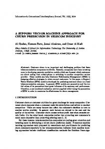
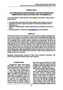
In practice, there are many unnatural patterns that may appear in industrial processes indicating out-of-control conditions. The typical unnatural patterns on control charts include trends, sudden shifts, mixtures, cyclic patterns, and systematic variation. A complete description of these unnatural patterns on control charts can be found in the Statistical Quality Control Handbook [1]. The most familiar multivariate processes monitoring and control procedure is the Hotelling T 2 chart for monitoring the mean vector of the processes. However, a recent study [5] indicated that unnatural patterns may appear on multivariate control charts. Fig. 1 depicts a sudden shift on control charts in a bivariate process with correlation coefficient ρ =0.5. Mason et al. [5] have proposed some visual methods to recognize patterns that occur in T 2 chart as summarized in Table 1. 6
3
UCL
0
_ X LCL
-3 -6
X2
X1
6
3
UCL
0
_ X LCL
-3 -6
1
8
16
24
32
1
8
16
24
32
Tsquared
24 18 UCL
12 6 0
1
8
16
24
32
Fig. 1. A sudden shift in a bivariate process ( ρ =0.5) Table 1. Patterns associated with a T 2 chart Pattern type Pattern that occurs in T 2 chart Trends T 2 values trend upward/downward Sudden shifts Distinct groupings of T 2 values Mixtures T 2 values clustered above zero line Cyclic patterns Repeated U shape (short period) Note: from [5].
2.2
Applications of Classification Techniques in Multivariate Processes
In the last few years, many researchers have investigated the application of artificial neural networks to multivariate statistical process control. Wang and Chen [6] developed a neural-fuzzy model not only to identify mean shifts but also to classify their magnitudes. Chen and Wang [7] also proposed a neural network approach for monitoring and classifying the mean shifts of multivariate process. Low et al. [8] presented a neural network procedure for detecting variance shifts in a multivariate process. Zorriassatine et al. [9] applied a neural network classification technique known as novelty detection to monitor
multivariate process mean and variance. Guh [10] designed a neural network-based model consists of two sequential modules that can identify and quantify the mean shifts in bivariate processes on-line. In recent years, the support vector machine has been introduced as a new technique for solving a variety of learning, classification and prediction problems. There is also some research on using support vector machines to monitor process variation [11-12]. The main purpose of this paper is to develop an efficient method to improve recognition of control chart patterns in multivariate processes. We implement two classifiers based on SVM and discriminant analysis to identify multivariate unnatural patterns. The discriminant analysis is used as a baseline for comparison. Furthermore, we also propose two alternative classification procedures for SVM-based classifier. The proposed approach will be demonstrated by multivariate processes with two and three quality characteristics.
3
Methodology
3.1
SVM-based Classifier
The support vector machine method is one of the most successful learning algorithms proposed in the applications of classification, regression and novelty detection tasks. SVM displays remarkable properties and generalization ability in these regions. SVM is a powerful machine learning tool that is capable of representing non-linear relationships and producing models that generalize well to unseen data. In practice, a classification task usually involves with training and testing data which consists of some data instances. Each instance in the training set contains one target value (class label) and several attributes (features). The goal of a classifier is to produce a model which predicts target value of data instances in the testing set which are given only the attributes. The basic concept of an SVM is to transform the data into a higher dimensional space and find the optimal hyperplane in the space that maximizes the margin between classes. The vectors near the hyperplane are defined as the support vectors. The main object of applying SVM for solving classification problems includes two steps. First, SVM transforms the input space to a higher dimensional feature space through a non-linear mapping function. Secondly, it constructs the separating hyperplane with maximum distance from the closest points of the training set. It has been shown that maximizing the margin of separation improves the generalization ability of the resulting classifier. A simple description of the SVM is provided here, for more details please refer to Burges [13]. Consider the problem of separating a set of examples (x1 , y1 ),..., (x i , yi ) iN=1 with N training vectors, where x i ∈ R d is the i th d -dimensional input vector (independent variables), yi ∈ {−1, + 1} is known target. The training of SVM involves the solution of quadratic optimization problem. Thus, the decision function can be written as yi ( w T φ ( x i ) + b) ≥ 1
(1)
In many practical applications, a separating hyperplane does not exist. In order to allow the possibility of examples violating Equation (1), the slack variables are restricted to ξ i ≥ 0 . It is important to note that the variables ξ i are introduced to allow for some classification errors. We are considering the mapping function φ represent a non-linear transformation to map the input vectors into a high-dimensional feature space. We rewrite the formula in order to relax the constraints as: yi (w T φ (x i ) + b) ≥ 1 − ξ i . Thus, the formula of quadratic optimization can be expressed as follows. min subject to
N 1 T w w + C ∑ξi 2 i =1 yi ( w T φ ( x i ) + b) ≥ 1 − ξ i ξi ≥ 0
(2)
where C is the penalty factor, w is the vector of hyperplane coefficients, b is a bias term and ξ i are parameters (errors) for handling nonseparable data. The index i labels the N training cases. We would like to emphasize that the parameter C determines the degree of penalty assigned to an error. It can be viewed as a tuning parameter which can be used to control the trade-off between maximizing the margin
and the classification error. Note that the larger the C , the more the error is penalized. Thus, C should be chosen with care to avoid over-fitting. The basic concept of SVM can be thought of as a balance between the term (1 / 2w T w ) and the training errors. Constructing a separating hyperplane in the feature space leads to a non-linear decision boundary in the input space. The costly calculation of dot products in a high-dimensional space can be avoided by introducing a kernel function satisfying K (x i , x j ) = φ (x i )φ (x j ) . The kernel function allows all necessary computations to be performed directly in the input space. Some popular kernel functions are defined in Table 2. Table 2. Kernel functions Kernel functions Comments Linear kernel K (x i , x j ) = x i x j Polynomial kernel of degree d K (x i , x j ) = (γ x i x j + r ) d , γ > 0 K (x i , x j ) = tanh((γ x i x j + r ), γ > 0 Sigmoid kernel Radial basis function kernel K (x i , x j ) = exp{−γ || x i − x j ||2 }, γ > 0 Note: γ , r , and d are referred to as kernel parameters.
The SVM was originally designed for binary classification problem. That is, the data is separated by a hyperplane defined by a number of support vectors. However, many real-world problems have more than two classes. Constructing multi-class SVM is still an on-going research issue [14]. Hsu and Lin [14] provided a comparison of methods for multi-class support vector machines. Basically, two types of approaches usually applied to multi-class classification problem in recent year. The first case, the SVM was modified in order to incorporate multi-class learning in the quadratic solving algorithm. That is, the SVM treat all classes at once considering only one optimization problem. Unfortunately, this approach can lead to a high computational cost. The second case, several binary SVM classifiers were combined. The one-against-all and one-against-one methods were used in the second case. The one-against-all method separates each class from all others and builds a combined classifier. For m -class problem, it constructs m binary SVMs. The i th SVM is trained with all the samples in the i th class with positive labels y = +1 , and all the other samples with negative labels y = −1 . The decision function chooses the class of a sample that corresponds to the maximum value of m binary decision functions specified by the furthest positive hyperplane. Thus, it uses a winner takes-all scheme. The one-against-all method is the earliest approach for multi-class SVM. Another method is the one-against-one which consists on a pairwise classification. The basic idea is to use m(m − 1) / 2 binary classifiers covering all pairs of classes instead of using only m classifiers as in the one-against-all. Each of the m(m − 1) / 2 binary SVMs casts one vote for its favored class, and finally the class with most votes wins. 3.2
Generation of Training Data Set in Multivariate Processes
In many industrial environments, there are a number of quality characteristics that need to be monitored simultaneously. The most commonly used statistics is the χ 2 statistic. Suppose that the p × 1 random vectors X1 , X 2 , …., X t , each representing the quality characteristics to be monitored, are observed over time. These vectors represent sample mean vectors from a sample of size n . The well-known χ 2 control chart is based on a measure of distance to the target mean vector of the process. For simplicity, it is assumed without loss of generality that the in-control process mean vector is μ 0 = (0, 0, 0..., 0)'= 0 . χ 2 statistic can be modeled as follows χ t2 = n( X t − μ 0 )' Σ −1 ( X t − μ 0 )
(3)
where Σ is a known covariance matrix. The upper limit on the control chart is UCL = χ α2 , p where χ α2 , p is the upper 100α percentage point of the χ 2 distribution with p degrees of freedom. When the in-control mean vector and covariance matrix are unknown, they are often replaced by the sample estimator, X and S , respectively. The test statistic for each sample that can be written as
Tt 2 = n( X t − X)' S −1 ( X t − X)
(4) 2
In this form, the control procedure is usually called the Hotelling T control chart. In practice, sufficient training examples of unnatural patterns may not be readily available. A common approach adopted by previous researches was to generate training examples based on predefined mathematical model [3], [15]. A p -dimensional multivariate normal process was simulated by generating pseudo-random variates from a multivariate normal distribution whose mean was μ and whose covariance matrix was a p × p matrix. For simplicity, it is assumed that the covariance matrix Σ is known. A natural (or random) pattern will be generated by a general form expressed as follows: Xt = μ + R t (5) where X t is the p quality characteristics observed at time t , μ represents a known process mean of the data series when the process is in control, R t is the random noise at time t . When a pattern occurs, a second noise component, d t , is introduced to the process mean of the errant variable(s). d t denotes a special disturbance at time t due to some assignable cause. By manipulating the value of d t , a pattern can then be simulated. In the research described here, four common unnatural patterns on control charts were considered, namely, trends, cyclic patterns, sudden shifts, and mixtures. All details in the generation of four types of d t are defined as follows. (1) Trends. The trends can be expressed as d t = θ t , where θ is the trend slope in terms of σ . (2) Sudden shifts. The sudden shifts can be written as d t = u δ , where u represent a parameter to determine the occurrence of shifting, u = 0 for non-shifting and u = 1 for shifting cases, respectively. The quantity δ can be defined as the magnitude of the mean shift in terms of σ . (3) Mixtures. The mixtures can be expressed as d t = (−1) ε Δ , where ε denotes a parameter to determine the appearance of shifting between distributions. The quantity ε will be controlled by a random number ν (ranges between 0 and 1) and the probability of shifting between distributions ( Pr ). The quantity ε = 0 if ν < Pr and ε = 1 if ν ≥ Pr . In this research Pr was fixed at 0.5. The quantity Δ can be defined as the offset from the process mean in terms of σ . (4) Cyclic patterns. The cyclic patterns can be modeled as d t = κ ⋅ sin( 2π t / Ω) , where κ is the amplitude of the cyclic patterns in terms of σ , and the symbol Ω is defined as the period of the cyclic pattern ( Ω =16 in this research). The simulation was implemented using Matlab software [16]. For simplicity, all variables were scaled such that each process variable has mean zero and variance one. With this approach, the covariance matrix is in correlation form; that is, the main diagonal elements are all one and the off-diagonal elements are the pairwise correlation ( ρ ) between the process variables. Note that the training examples of large shifts will include some in-control data followed by shifted data (i.e., partially shifted data). The parameters (in terms of σ ) used for simulating patterns are summarized in Table 3. Note that in-control data are also included in the training set. We also considered multivariate processes with various positive and negative correlation coefficients to cover the whole range of parameters for each pattern type. Table 3. Parameters of training examples for unnatural patterns Pattern type Parameters No. of training cases Natural In-control data 3000 Trend gradient: 0.10, 0.125, 0.15 3000 Sudden shift shift magnitude: 1.5, 2.0, 3.0 3000 Mixture magnitude: 2.0, 2.5, 3.0 3000 Cyclic pattern amplitude: 1.5, 2.0, 3.0; period: 16 3000
In this investigation, the interpretations of errant variable(s) were described as follows. Take p =3 as an example, the occurrence of unnatural patterns was assumed to occur in one of the following ways. (1) One errant variable only. Only one of the variables incurred unnatural pattern. (2) Two errant variables. Two of the variables incurred unnatural pattern while the other variable remains in-control situation. (3) All three errant variables. All variables incurred the same unnatural pattern types and magnitudes.
3.3
Selection of Input Vector
The representation of the data in the training set has an intense influence upon the performance of classifier. Note that determination of an adequate window size is one of the critical steps in the current application. Since quick computation is of most importance for process control, it is desirable to lessen the size of window to obtain an efficient calculation. Preliminary studies indicated that a too small window size might generate a higher Type I error due to insufficient information to represent the features of the data. On the other hand, a large window size may need a long computation time. In the current research, a window size of 32 was chosen through experimentation. Thus, we calculated 32 T 2 statistics as the components of the feature vector. 3.4
Model Selection and Training
Although support vector machines have shown great generalization performance in a number of applications, one problem that faces the user of an SVM is how to choose a kernel and the specific parameters for that kernel. The kernel functions map the original data into higher-dimension space and make the input data set linearly separable in the transformed space. The choice of kernel functions is highly problem-dependent and it is the most important factor in support vector machine applications. In our classification task, four different kernel functions from Table 2 are used and compared in terms of their classification performances for the selection of kernel function. Consequently, the best performance is obtained with a radial basis function (RBF) and it is by far the most popular choice of kernel types used in support vector machines. Hence, in our implementation, we chose the RBF kernel as our kernel function in order to achieve better performance. As mentioned previously, the use of SVM involves training and testing procedures, with a particular kernel function, which in turn has specific kernel parameters. For RBF kernel function, the parameters must be determined are the kernel parameter γ and the penalty factor C . Kernel parameter defines the structure of the high dimensional feature space where a maximal margin hyperplane will be found. The SVM parameters are usually selected through experimentation. The parameter C controls the trade off between maximizing the margin and classifying the training set without error. The larger the C , the more the error is penalized. The penalty factor C should be chosen with caution to avoid over-fitting. In determining these two parameters, a 10-fold cross-validation experiment was used to choose parameters that yield the best result. That is, we divided the training set into 10 subsets. Then, we performed the tests for the 10 runs, each with a different subset as the test set and with the union of the other nine subsets as the training set. The cross-validation was carried out in two stages. In the first stage, a search was made for an estimate of the penalty factor C and the kernel parameter γ that achieves the highest classification accuracy. In the second phase of training, the estimated values of these two parameters were used to train an SVM model using the entire training samples. Subsequently, this set of parameters was applied to the test dataset. A grid-search on C and γ were recommended for using cross-validation. The pairs of C and γ were tried and the one with the best cross-validation accuracy was picked in practice. In this work, values for γ and C were checked in the [0.03125, 2] and [2, 40] ranges, respectively. Different parameter settings will be used for data with different ρ values. In this investigation, SVM was implemented in STATISTICA software [17]. 3.5
Two Procedures for Out-of-control Signal Detection and Classification
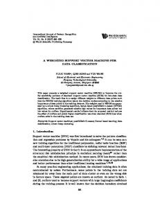
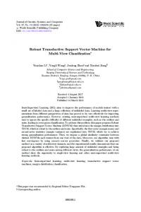
In this paper, two alternative schemes are proposed to construct multivariate unnatural pattern recognizers. The first scheme (referred to as one-stage classification procedure) comprises an SVM-based classifier (or the discriminant analysis) that is designed and trained to recognize patterns in multivariate processes at a time. The training inputs consist of unnatural patterns and in-control data. As Fig. 2(a) indicates, the number of class m is set to 5, i.e., yi ∈ {1, 2, 3, 4,5} . The second scheme of classification (referred to as Two-stage classification procedure) contains two SVMs in series, SVM-I and SVM-II, as shown in Fig. 2(b). The SVM-I works as a detector. When an out-of-control signal is detected, the SVM-II classifier is employed to identify which type of unnatural pattern for the detected signal. For SVM-I, the output class m is set to 2. For SVM-II classifier, the
number of class m is set to 4, representing four types of unnatural patterns.
Fig. 2. Architectures of two procedures
4
Results and Discussion
4.1
Performance Evaluation
In the evaluation process, the rate of correct classification (ROCC) was calculated. The testing samples were generated in the same way as training samples in this experiment. Each of classifiers was tested by 75000 testing samples (five times the quantities of training samples). The range of parameters used for simulating unnatural patterns was given in Table 3. Similarly, each pattern type was tested with various positive and negative correlation coefficients in multivariate processes, respectively. The various average rate of ROCC were measured and based on 10000 simulation runs at each change magnitude. The discriminant analysis in multivariate statistics is used as a baseline for comparison. Discriminant analysis is a multivariate technique concerned with separating distinct sets of observations and with allocating new observations to previously defined groups [18]. In this experiment, discriminant analysis was implemented in Minitab software [19]. The quadratic function was selected due to its superior performance. 4.2
Performances of Different Classifiers
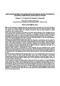
In this session, we will discuss the performances of the proposed classifier in multivariate processes. Two classifiers based on SVM and discriminant analysis that used same input dataset for comparison. The performances of discriminant analysis are selected as the baseline. The results are reported for one-stage classification procedure with various ρ ' s . Fig. 3 reveals overall performances of SVM and discriminant analysis for one-stage classification procedure. The resulting values are plotted in Fig. 3(a) for p =2 in “one errant variable only” case. We can observe that SVM-based classifiers yield more stable results than discriminant analysis with various positive and negative correlation coefficients. It is worth noting that SVMs or discriminant analysis methods provide better performance for ρ =-0.9 and 0.9. The lowest average classification accuracy occur in ρ =-0.1 and 0.1. A close look at the results reveals that the SVM-based pattern recognizer has the same capability in detecting different directions of ρ changes. As mentioned above, the curve becomes “U” shape in Fig. 3(a), which is different from Fig. 3(b). That is, for “two errant variables” case, the classification performance improves as the value of ρ decreases. From this figure, the results lead to the conclusion that SVM-based classifiers are superior to traditional discriminant analysis techniques.
Classif iaction accuracy
95 90 85 80 75
Variable SVM DA
100 Classif iaction accuracy
Variable SVM DA
100
95 90 85 80 75
-0.9 -0.7 -0.5 -0.3 -0.1 0.1
0.3 0.5
0.7
0.9
-0.9 -0.7 -0.5 -0.3 -0.1 0.1 0.3
Correlation coef f icient
(a) p=2, one errant variable only
0.5 0.7 0.9
Correlation coef f icient
(b) p=2, tw o errant variables
Fig. 3. Overall performances for one-stage classification procedure Table 4. Overall performances of classifiers for different change types ( p =3) ρ SVM increment% SVM Discriminant analysis Unnatural type 0.1 091.53 /091.43 086.51 /085.86 5.02 / 5.57 0.3 093.75 /093.48 089.17 /088.65 4.58 / 4.83 One errant 093.27 /092.93 3.37 / 3.50 0.5 096.64 /096.43 variable only 097.69 /097.51 1.59 / 1.73 0.7 099.28 /099.24 0.27 / 0.30 0.9 100.00 /100.00 099.73 /099.70 096.01 /095.36 2.39 / 2.73 0.1 098.40 /098.09 0.3 097.86 /097.78 095.41 /095.15 2.45 / 2.63 Two errant 096.80 /096.29 1.83 / 2.22 0.5 098.63 /098.51 variables 098.56 /098.36 1.07 / 1.26 0.7 099.63 /099.62 0.23 / 0.29 0.9 100.00 /100.00 099.77 /099.71 098.03 /097.88 1.24 / 1.43 0.1 099.27 /099.31 0.3 098.33 /097.94 096.13 /095.65 2.20 / 2.29 All three errant 092.99 /092.53 3.27 / 3.65 0.5 096.26 /096.18 variables 089.90 /089.49 4.29 / 4.35 0.7 094.19 /093.84 087.42 /086.53 4.25 / 4.92 0.9 091.67 /091.45 Note: (a/b) denotes (training/test).
For p =3, the overall performances of SVM and discriminant analysis for different change types with ρ > 0 are displayed in Table 4. From the results, we observe a relation between correlation coefficient ρ and classification accuracy. For “one errant variable only” and “two errant variables” situations, the classification accuracies improve as the value of ρ increases. On the contrary, the classification performance worsens as the value of ρ increases in “all three errant variables” situation. The same observations hold for discriminant analysis. 4.3
Comparison of Different Classification Procedures
The comparisons of classification accuracy with two alternative classification procedures are presented in this session. Table 5 provides the confusion matrix of classification results for “one errant variable only” situation with various ρ ’s. The rows in the confusion matrix represent the desired results (i.e. trend, sudden shift, mixture, cyclic pattern), while columns indicate the output as recognized by classifier. Entries (in boldface) along the diagonal indicate correct classification; while off-diagonal entries would represent that the unnatural patterns have been misclassified as the wrong type of classes. We can observe that there is a strong agreement between training and testing results, indicating no over-fitting problems with SVMs. Table 5. Confusion matrix of SVM with various ρ ’s for two-stage classification procedure ( p =2, one errant variable only) Recognized patterns ρ Input patterns Trend Sudden shift Mixture Cyclic pattern Trend 000.03 /000.01 000.00 /000.00 000.00 /000.00 0.9 099.97 /099.99 Sudden shift 000.00 /000.00 000.00 /000.00 000.00 /000.00 100.00 /100.00 Mixture 000.00 /000.00 000.00 /000.00 000.00 /000.01 100.00 /100.00
Cyclic pattern 000.00 /000.00 Trend 0.5 095.90 /095.19 Sudden shift 002.35 /002.26 Mixture 000.03 /000.16 Cyclic pattern 000.00 /000.03 Trend 0.1 091.73 /092.00 Sudden shift 004.10 /003.95 Mixture 000.43 /000.50 Cyclic pattern 000.11 /000.07 Trend -0.1 092.57 /092.54 Sudden shift 003.86 /004.65 Mixture 000.53 /000.59 Cyclic pattern 000.14 /000.07 Trend -0.5 095.53 /094.92 Sudden shift 002.18 /002.34 Mixture 000.30 /000.12 Cyclic pattern 000.00 /000.01 Trend -0.9 099.97 /099.96 Sudden shift 000.00 /000.00 Mixture 000.00 /000.00 Cyclic pattern 000.00 /000.00 Note: (a/b) denotes (training/test).
000.03 /000.00 003.90 /004.69 096.55 /096.64 000.03 /000.11 001.85 /001.54 007.77 /007.46 093.48 /093.13 000.30 /000.31 002.88 /002.73 006.93 /007.01 094.00 /092.59 000.17 /000.31 003.40 /002.94 004.27 /004.99 096.66 /096.57 000.07 /000.08 001.17 /001.83 000.03 /000.04 100.00 /100.00 000.00 /000.00 000.00 /000.00
099.97 /100.00 000.00 /000.03 001.09 /001.08 001.47 /001.31 098.01 /098.08 000.13 /000.12 002.38 /002.86 002.13 /002.47 096.20 /096.30 000.23 /000.16 002.07 /002.67 001.80 /002.35 095.02 /096.10 000.03 /000.03 001.16 /001.06 001.40 /001.25 098.59 /097.83 000.00 /000.00 000.00 /000.00 000.00 /000.00 100.00 /100.00
Variable 1-stage 2-stage
100
Classification accuracy
000.00 /000.00 000.20 /000.09 000.00 /000.01 098.47 /098.42 000.14 /000.35 000.37 /000.42 000.04 /000.06 097.13 /096.72 000.82 /000.91 000.27 /000.29 000.07 /000.09 097.50 /096.75 001.43 /000.89 000.17 /000.07 000.00 /000.02 098.23 /098.55 000.24 /000.33 000.00 /000.00 000.00 /000.00 100.00 /100.00 000.00 /000.00
95
90
85
80 -0.9 -0.7 -0.5 -0.3 -0.1 0.1 0.3
0.5
0.7 0.9
Correlation coefficient
Fig. 4. Overall performances of SVMs for different classification procedures ( p =2, one errant variable only)
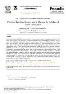
Fig. 4 illustrates the overall performances of SVMs for two types of classification procedures in bivariate processes ( p =2). For “one errant variable only” case, we can observe that two-stage classification procedure of SVM yields better results than that of one-stage approach. As Fig. 4 indicates, the SVM-based pattern recognizer has the same capability in detecting different directions of ρ changes. Table 6 summarizes the overall performances of SVMs for two types of procedures in multivariate processes with p =3. As we can see, the two-stage classification procedure performs markedly better than one-stage approach. Table 6. Overall performances of SVM for different classification procedures ( p =3) One-stage classification Two-stage classification Unnatural ρ Increment % procedure procedure type 0.1 090.39 /090.34 093.27 /093.06 02.88 /02.72 One errant 0.3 092.87 /092.55 095.07 /094.79 02.20 /02.24 variable 0.5 096.04 /095.86 097.39 /097.15 01.35 /01.29 0.7 099.12 /099.10 099.37 /099.31 00.25 /00.21 only 0.9 100.00 /100.00 100.00 /100.00 00.00 /00.00 0.1 099.13 /099.15 099.30 /099.36 00.17 /00.21 All three 0.3 097.98 /097.56 098.49 /098.20 00.51 /00.64 errant 0.5 095.63 /095.56 096.93 /096.73 01.30 /01.17 0.7 093.26 /092.98 095.07 /094.94 01.81 /01.96 variables 092.93 /092.89 02.40 /02.61 0.9 090.53 /090.28 Note: (a/b) denotes (training/test).
4.4
Sensitivity of SVM to Parameters
In this section, we would like to investigate the effects of changing two important parameters on the results of SVM. Table 7 gives the results of SVMs at various combinations of C and γ with correlation coefficient ρ =0.7. It is evident that different parameter combinations yield quite stable results. These results lead to the conclusion that SVMs are quite robust against parameter selections. Table 7. Sensitivity of SVM to parameters with correlation coefficient ρ =0.7 ( p =2, one errant variable only)
C \γ
0.03125 0.0625 2 98.53/98.58 98.72/98.87 5 98.79/98.90 98.97/99.02 10 98.96/99.00 99.12/99.09 20 99.08/99.06 99.16/99.15 40 99.11/99.12 99.21/99.17 Note: (a/b) denotes (training/test).
5
0.125 98.97/99.04 99.16/99.11 99.16/99.18 99.22/99.18 99.27/99.18
0.25 99.13/99.13 99.19/99.18 99.26/99.20 99.33/99.19 99.45/99.22
0.5 99.21/99.19 99.30/99.22 99.43/99.22 99.53/99.25 99.61/99.23
1.0 99.35/99.26 99.49/99.26 99.62/99.29 99.72/99.24 99.80/99.19
2.0 99.52/99.28 99.68/99.27 99.77/99.23 99.86/99.20 99.91/99.14
Conclusions
In multivariate SPC, developing an efficient approach for recognition of control chart patterns is a critical issue. In this paper, we have proposed an SVM-based approach for control charts pattern recognition in multivariate processes. Different shift scenarios were addressed by various covariance matrices. The performances of competing classifiers were evaluated by estimating the average classification accuracy. Extensive comparisons show that the SVM-based classifier outperforms the traditional discriminant analysis. Furthermore, we also propose two alternative classification procedures for SVM-based classifier. Simulation results have shown that the SVM-based classifier can be further improved by the two-stage classification procedure.
References 1.
Western Electric Company: Statistical Quality Control Handbook. Western Electric Co. Indiana Indianapolis (1958) 2. Nelson, L. S.: The Shewhart control chart-tests for special cause. Journal of Quality Technology. 16 (1984) 237-239 3. Cheng, C. S.: A neural network approach for the analysis of control chart patterns. International Journal of Production Research. 35 (1997) 667-697 4. Montgomery, D. C.: Introduction to statistical quality control. 5th edn. John Wiley & Sons, New Jersey (2005) 5. Mason, R. L., Chou, Y.-M., Sullivan, J. H., Stoumbos, Z. G., Young, J. C.: Systematic patterns in T 2 charts. Journal of Quality Technology. 35 (2003) 47-58 6. Wang, T. Y., Chen, L. H.: Mean shifts detection and classification in multivariate process: a neural-fuzzy approach. Journal of Intelligent Manufacturing. 13 (2002) 211-221 7. Chen, L.-H., Wang, T.-Y.: Artificial neural networks to classify mean shifts from multivariate χ 2 chart signals. Computers & Industrial Engineering. 47 (2004) 195-205 8. Low, C., Hsu, C. M., Yu, F. J.: Analysis of variations in a multi-variate process using neural networks. International Journal of Advanced Manufacturing Technology. 22 (2003) 911-921 9. Zorriassatine, F., Tannock, J. D. T., O’Brien, C.: Using novelty detection to identify abnormalities causes by mean shifts in bivariate processes. Computers and Industrial Engineering. 44 (2003) 385-408 10. Guh, R. S.: On-line identification and quantification of mean shifts in bivariate processes using a neural network-based approach. Quality and Reliability Engineering International. 23 (2007) 367–385 11. Chinnam, R. B.: Support vector machines for recognizing shifts in correlated and other manufacturing processes. International Journal of Production Research. 40 (2002) 4449-4466 12. Sun, R., Tsung, F.: A kernel-distance-based multivariate control chart using support vector methods.
International Journal of Production Research. 41 (2003) 2975-2989 13. Burges, C. J. C.: A tutorial on support vector machines for pattern recognition. Data Mining and Knowledge Discovery. 2 (1998) 121-167 14. Hsu, C.-W., Lin, C.-J.: A comparison of methods for multiclass support vector machines. IEEE Transactions on Neural Networks. 13 (2002) 415-425 15. Guh, R. S., Hsieh, Y. C.: A neural network based model for abnormal pattern recognition of control charts. Computers & Industrial Engineering, 36 (1999) 97-108 16. MathWorks.: MATLAB 7.0 User’s Guide. MathWorks, Natick (2004) 17. STATISTICA.: STATISTICA Data Miner. StatSoft, Oklahoma Tulsa (2003) 18. Johnson, R. A., Wichern, D. W.: Applied Multivariate Statistical Methods. 5th edn. Prentice Hall, New Jersey (2002) 19. Minitab.: Minitab 14.0 User’s Guide. Minitab, U.S. (2004)