Apr 29, 2011 - We then apply our test to a data set provided by Tecator, which consists of ... µ = E(Yn) and (1.1) reduces to the functional linear model. Yn = µ +.
A test of significance in functional quadratic regression 1 Lajos Horv´ath and Ron Reeder Department of Mathematics, University of Utah
arXiv:1105.0014v1 [math.ST] 29 Apr 2011
Abstract We consider a quadratic functional regression model in which a scalar response depends on a functional predictor; the common functional linear model is a special case. We wish to test the significance of the nonlinear term in the model. We develop a testing method which is based on projecting the observations onto a suitably chosen finite dimensional space using functional principal component analysis. The asymptotic behavior of our testing procedure is established. A simulation study shows that the testing procedure has good size and power with finite sample sizes. We then apply our test to a data set provided by Tecator, which consists of near-infrared absorbance spectra and fat content of meat. Keywords: Absorption spectra; Asymptotics; Functional data analysis; Polynomial regression; Prediction; Principal component analysis.
1
Introduction and results
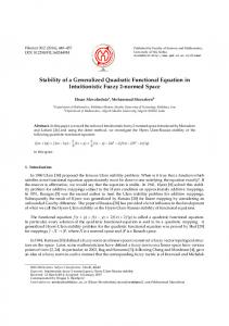
In a predictive model, it may be more natural and appropriate for certain quantities to be represented as trajectories rather than a single number (Kirkpatrick and Heckman, 1989). For example, a young animal’s size may be considered as a function of time, giving a growth trajectory. A model to predict a certain response from growth trajectories is useful to animal breeders because they may be able to produce more valuable animals by changing their growth patterns (Fitzhugh, 1976). M¨ uller and Zhang (2005) used egg-laying trajectories from Mediterranean fruit flies to predict a female fly’s remaining lifetime. Frank and Friedman (1993) and Wold (1993) provide an early discussion on the applications of principal components to analyze curves in chemistry. Yao and M¨ uller (2010) and Borggaard and Thodberg (1992) used absorbance trajectories to predict the fat content of meat samples. The absorbance at any particular wavelength is a measurement related to the proportion of light that passes through a meat sample. A representative sample of 15 of the 240 absorbance trajectories are pictured in Figure 1. In functional regression, special attention has been given to functional linear models (Cardot et al., 2003; Shen and Faraway, 2004; Cai and Hall, 2006; Hall and Horowitz, 2007). However, it is pointed out in Yao and M¨ uller (2010) that this model imposes a constraint on the regression relationship that may not be appropriate in some scenarios. Yao and M¨ uller (2010) generalized this to a functional polynomial model, which has greater flexibility. In functional polynomial regression, as in standard polynomial regression, one must balance the costs and benefits of using more parameters in the model. In this paper, we will develop a 1
Research partially supported by NSF grant DMS 0905400
1
Figure 1: Absorbance trajectories from 15 samples of finely chopped pure meat. test to determine if a quadratic term is justified in the model or if a functional linear model adequately describes the regression relationship. The functional quadratic model in which a scalar response, Yn , is paired with a functional predictor, Xn (t), is defined as Z 1 Z 1Z 1 c k(t)Xn (t) dt + h(s, t)Xnc (s)Xnc (t) dt ds + εn , Yn = µ + (1.1) 0
0
0
Xnc (t)
where = Xn (t) − E (Xn (t)) is the centered predictor process. If h(s, t) = 0, then µ = E(Yn ) and (1.1) reduces to the functional linear model Z 1 Yn = µ + k(t)Xnc (t) dt + εn . (1.2) 0
Cardot and Sarda (2011) and Mas and Pumo (2011) point out in their survey papers that since we can choose a function in (1.2), the functional linear model can be used in a large variety of applications. The functional linear model provides a very simple relation between Xn (t) and Yn , so it is important to check if the more involved quadratic model (1.1) provides a real improvement. In other words, one should test whether the quadratic term is really needed. To test the significance of the quadratic term in (1.1), we test the null hypothesis, H0 : h(s, t) = 0, against the alternative HA : h(s, t) 6= 0. 2
(1.3)
To reduce the dimensionality and avoid overfitting in our functional regression model, we will project the predictor process onto a suitably chosen finite dimensional space. The space is spanned by the eigenfunctions of C(t, s) = E(Xn (t) − µX (t))(Xn (s) − µX (s)), the covariance function of the predictor process, where µX (t) = EXn (t). We will denote the eigenfunctions and associated eigenvalues by {(vi (t), λi ), 1 ≤ i ≤ ∞}. We can and will assume that λi is the ith largest eigenvalue and that the eigenfunctions are orthonormal. It is clear that we can assume that h is symmetric, and we also impose the condition that the kernels are in L2 : Z 1Z 1 h2 (s, t)dtds < ∞, (1.4) h(s, t) = h(t, s) and 0
Z
0
1
k 2 (t)dt < ∞.
(1.5)
0
Thus we have the expansions h(s, t) = =
∞ X ∞ X
ai,j vj (s)vi (t)
i=1 j=1 ∞ X
∞ X ∞ X
i=1
i=1 j=i+1
ai,i vi (s)vi (t) +
and k(t) =
∞ X
(1.6) ai,j (vj (s)vi (t) + vi (s)vj (t))
bi vi (t).
(1.7)
i=1
By projecting onto the space spanned by {v1 , . . . , vp } and using (1.6) and (1.7), we can write the model (1.1) as Yn = µ +
p X i=1
bi hXnc , vi i
p p X X + (2 − 1{i = j})ai,j hXnc , vi ihXnc , vj i + ε∗n ,
(1.8)
i=1 j=i
where ε∗n
=
∞ X
∞ X ∞ X c εn + bi hXn , vi i+ (2−1{i i=p+1 i=p+1 j=i
=
p ∞ X X
j})ai,j hXnc , vi ihXnc , vj i+
2ai,j hXnc , vi ihXnc , vj i.
i=1 j=p+1
We note that (1.8) is written as a standard linear model, but the error term, ε∗n , and the design points, {hXnc , vi i, 1 ≤ i ≤ p}, are dependent. Unfortunately, we cannot use (1.8) directly for statistical inference since vi (t) and µX (t) are unknown. We estimate µX (t) and C(t, s) with the corresponding empiricals N 1 X ¯ Xn (t) X(t) = N n=1
and
N X � � ˆ s) = 1 ¯ ¯ C(t, Xn (t) − X(t) Xn (s) − X(s) . N n=1
3
ˆ1 ≥ λ ˆ2 ≥ . . . ˆ s) are denoted by λ The eigenvalues and the corresponding eigenfunctions of C(t, and vˆ1 , vˆ2 , . . . . Eigenfunctions corresponding to unique eigenvalues are uniquely determined up to signs. For this reason, we cannot expect more than to have cˆi vˆi (t) be close to vi (t), where the cˆi ’s are random signs. We replace equation (1.8) with Yn = µ+
p X
¯ cˆi vˆi i+ bi hXn − X,
i=1
p p X X
¯ cˆi vˆi ihXn − X, ¯ cˆj vˆj i+ε∗∗ (2−1{i = j})ai,j hXn − X, n , (1.9)
i=1 j=i
where ε∗∗ n
=ε∗n
+ p
−
p X
bi hXnc , vi
− cˆi vˆi i +
i=1 p
XX
p X
¯ − µX , cˆi vˆi i bi hX
i=1
� ¯ cˆi vˆi ihXn − X, ¯ cˆj vˆj i − hX c , vi ihX c , vj i . (2 − 1{i = j})ai,j hXn − X, n n
i=1 j=i
We can write (1.9) in the concise form ˜ A ˆ B ˜ + ε∗∗ , Y=Z µ
(1.10)
where �T Y = Y1 , Y2 , . . . , YN , � ˜ = cˆ1 b1 , cˆ2 b2 , . . . , cˆp bp T , B
� ˜ = vech {ˆ A ci cˆj ai,j (2 − 1{i = j}) , 1 ≤ i ≤ j ≤ p}T , � ∗∗ T ∗∗ , ε∗∗ = ε∗∗ 1 , ε2 , . . . , εN
and ˆT 1 ˆT F D 1 1 D T ˆ T 1 ˆ2 F 2 ˆ Z= . . . . . . . . . ˆT 1 ˆT F D N N
with � ˆ n = vech {hˆ ¯ vj , Xn − Xi, ¯ 1 ≤ i ≤ j ≤ p}T , D vi , Xn − Xihˆ � ¯ vˆ1 i, hXn − X, ¯ vˆ2 i, . . . , hXn − X, ¯ vˆp i T . ˆ n = hXn − X, F The half-vectorization, vech(·), stacks the columns of the lower triangular portion of the matrix under each other. Although we write our model in the form of a general linear model, ˆ it is important to note that it is not a classical linear model. First, ε∗∗ is correlated with Z ∗∗ because ε contains additional error terms which come from projecting onto a p-dimensional space. Another important difference between (1.10) and a classical linear model is that the ˜ and B, ˜ are random; they depend on the random signs, cˆi . We parameters to be estimated, A ˜ ˜ estimate A, B, and µ using the least squares estimator: ˆ A � �−1 ˆT Z ˆ ˆ T Y. B ˆ = Z Z (1.11) µ ˆ 4
ˆ and B, ˆ we will use the notation that A ˆ = vech({ˆ To represent elements of A ai,j (2 − 1{i = � T ˆ = ˆb1 , ˆb2 , . . . , ˆbp . j}), 1 ≤ i ≤ j ≤ p}T ) and B ˆ will be close to zero since A ˜ is zero. If H0 is not correct, we We expect, under H0 , that A ˆ to be relatively large. This suggests that a testing procedure could expect the magnitude of A ˆ Due to the random signs coming from the estimation of the eigenfunctions, A ˆ be based on A. will not be asymptotically normal. However, if the random signs are “taken out,” asymptotic ˆ with some normality can be established. Hence our test statistic will be a quadratic form of A random weight matrices. Let N X ˆ T, ˆ nD ˆ = 1 D G n N n=1 N X ˆ = 1 ˆ n, M D N n=1
and
N 1 X 2 τˆ = εˆ , N n=1 n 2
where εˆn = Yn − µ ˆ−
p X
ˆbi hXn − X, ¯ vˆi i −
p p X X ¯ vˆi ihXn − X, ¯ vˆj i (2 − 1{i = j})ˆ ai,j hXn − X,
i=1
i=1 j=i
are the residuals under H0 . We reject the null hypothesis if UN =
N ˆT ˆ ˆM ˆ T )A ˆ A (G − M τˆ2
is large. The main result of this paper is the asymptotic distribution of UN under the null hypothesis. First, we discuss the assumptions needed to establish asymptotics for UN : Assumption 1.1. {Xn (t), n ≥ 1} is a sequence of independent, identically distributed Gaussian processes. Assumption 1.2. �Z E
�4
1
Xn2 (t) dt
< ∞.
0
Assumption 1.3. {εn } is a sequence of independent, identically distributed random variables satisfying Eεn = 0 and Eε4n < ∞, and Assumption 1.4. the sequences {εn } and {Xn (t)} are independent. The last condition is standard in functional data analysis. It implies that the eigenfunctions v1 , v2 , . . . , vp are unique up to a sign. 5
Assumption 1.5. λ1 > λ2 > · · · > λp+1 . Theorem 1.1. If H0 , (1.5) and Assumptions 1.1–1.5 are satisfied, then D
UN −→ χ2 (r), ˆ where r = p(p + 1)/2 is the dimension of the vector A. The proof of Theorem 1.1 is given in Section 4. Remark 1.1. By the Karhunen-Lo`eve expansion, every centered, square integrable process, Xnc (t), can be written as ∞ X c Xn (t) = ξn,` ϕ` (t), `=1
where ϕ` are orthonormal functions. Assumption 1.1 can be replaced with the requirement that 3 ξn,1 , ξn,2 , . . ., ξn,p are independent with Eξn,` = 0 and Eξn,` = 0 for all 1 ≤ ` ≤ p. Our last result provides a simple condition for the consistency of the test based on UN . Let A = vech({ai,j (2 − 1{i = j}), 1 ≤ i ≤ j ≤ p}T ), i.e. the first r = p(p + 1)/2 coefficients in the expansion of h in (1.6). Theorem 1.2. If (1.4), (1.5), Assumptions 1.1–1.5 are satisfied and A 6= 0, then we have that P UN −→ ∞. The condition A 6= 0 means that h is not the 0 function in the space spanned by the functions vi (t)vj (s), 1 ≤ i, j ≤ p.
2
A simulation study
In this section, we investigate the empirical size and power of the testing procedure for finite sample sizes. Seeking to obtain a test of size α = .01, .05, or .10, a rejection region was chosen according to the limiting distribution of the test statistic. Since the limiting distribution is χ2 (r), the rejection region is (∆, ∞), where P (χ2 (r) > ∆) = α. Simulated data was then used to compute the outcome of the test statistic. Iterating this procedure 5,000 times, we kept track of the proportion of times that the outcome fell in the predetermined rejection region. When simulations are done under H0 , this gives us the empirical size of the test, which we expect to be close to the nominal size, α, for large sample sizes. When simulations are done under the alternative, HA , the proportion gives us the empirical power of the test. In our first simulation study, the εn ’s were generated according to the distribution of independent standard normals. We generated the Xn (t)’s according to the distribution of independent standard Brownian motions. Then, using k(t) = 1 and h(s, t) = c, we obtained Yn according to (1.1). Thus the power of the test is a function of the parameter c. In particular, when c = 0, the null hypothesis is true. The resulting empirical size and power are given in Table 1. 6
The distribution of our test statistic has been shown to converge to a χ2 (r). Thus we expect the empirical and nominal size to be close for samples of size N = 200 and even closer when N = 500, as observed in Table 1. Since our testing procedure depends on the choice of how many principal components to keep, results are given in Table 1 for p = 1, 2, and 3. One possible method of selecting p is to follow the advice of Ramsay and Silverman (2005) and choose p so that approximately 85% of the variance within a sample is described by the first p principal components. Although Theorem 1.1 is proven under the assumption that Xn (t) is a Gaussian process, the result of Theorem 1.1 holds under relaxed conditions as discussed in Remark 1.1. We will now investigate the empirical size and power of our test when Xn (t) is not a Gaussian process. We generate the εn ’s according to a uniform distribution on (−0.5, 0.5). The predictors, Xn (t), are generated according to Xn (t) = (T1,n + T2,n t + T3,n (2t2 − 1) + T4,n (4t3 − 3t)) /4, where {Ti,n , 1 ≤ i ≤ 4, 1 ≤ n} are iid random variables having a t-distribution with 5 degrees of freedom. The polynomials in the definition of Xn (t) are the orthogonal Chebyshev polynomials. The resulting empirical size and power are given in Table 2. We see from Table 2 that our testing procedure is robust against non-Gaussian observations. Comparing Tables 1 and 2, we see that the value of the test statistics tends to be larger if the Xn ’s are not normally distributed for small N . The overrejection fades as N gets larger so in case of non-Gaussian Xn ’s, larger sample sizes are needed. This also explains the somewhat better power of the procedure in the case of non-Gaussian errors.
3
Application to spectral data
In this section we apply our test to the data set collected by Tecator and available at http://lib.stat.cmu.edu/datasets/tecator. Tecator used 240 samples of finely chopped pure meat with different fat contents. For each sample of meat, a 100 channel spectrum of absorbances was recorded using a Tecator Infratec food and feed analyzer. These absorbances can be thought of as a discrete approximation to the continuous record, Xn (t). Also, for each sample of meat, the fat content, Yn was measured by analytic chemistry. The absorbance curve measured from the nth meat sample is given by Xn (t) = log10 (I0 /I), where t is the wavelength of the light, I0 is the intensity of the light before passing through the meat sample, and I is the intensity of the light after it passes through the meat sample. The Tecator Infratec food and feed analyzer measured absorbance at 100 different wavelengths between 850 and 1050 nanometers. This gives the values of Xn (t) on a discrete grid from which we can use cubic splines to interpolate the values anywhere within the interval. A representative sample of 15 of the 240 absorbance trajectories are pictured in Figure 1. Yao and M¨ uller (2010) proposed using a functional quadratic model to predict the fat content, Yn , of a meat sample based on its absorbance spectrum, Xn (t). We are interested in determining whether the quadratic term in (1.1) is needed by testing its significance for this data set. From the data, we calculate U240 . The p-value is then P (χ2 (r) > U240 ). The test statistic and hence the p-value are influenced by the number of principal components that we choose to keep. If we select p according to the advice of Ramsay and Silverman (2005), we will keep only p = 1 principal component because this explains more than 85% of the variation between absorbance curves in the sample. Table 3 gives p-values obtained using p = 1, 2, 7
and 3 principal components, which strongly supports that the quadratic regression provides a better model for the Tecator data. Table 1: Empirical power of test (in %) based on 5,000 simulations using iid Brownian motions for Xn (t) and iid standard normals for εn . α = .01 c N = 200 N = 500 p=1 p=2 p=3 p=1 p=2 p=3 0.0 1.02 1.37 1.95 1.10 1.30 1.15 0.2 10.81 6.87 6.52 30.35 20.35 12.85 0.4 49.51 37.24 29.76 91.90 84.25 74.35 0.6 86.68 77.74 70.19 100.00 99.70 98.75 0.8 98.50 96.05 92.98 100.00 100.00 100.00 1.0 99.94 99.57 99.05 100.00 100.00 100.00
α = .05 c 0.0 0.2 0.4 0.6 0.8 1.0
N = 200 p=1 p=2 5.15 6.00 25.90 19.17 72.10 60.31 95.21 90.43 99.60 98.90 99.99 99.87
N = 500 p=3 p=1 p=2 p=3 7.44 5.60 5.75 6.05 18.02 53.05 40.00 31.35 50.38 97.90 93.70 88.55 85.77 100.00 99.90 99.60 97.60 100.00 100.00 100.00 99.84 100.00 100.00 100.00
α = .10 c 0.0 0.2 0.4 0.6 0.8 1.0
p=1 10.27 36.60 80.89 97.60 99.85 99.99
N = 200 p=2 11.18 29.50 71.08 94.77 99.47 99.95
p=3 p=1 13.35 10.60 27.03 65.00 62.27 99.30 90.91 100.00 98.57 100.00 99.91 100.00
8
N = 500 p=2 p=3 11.05 11.55 52.45 43.75 96.60 93.10 99.95 99.75 100.00 100.00 100.00 100.00
Table 2: Empirical power of test (in %) based on 5,000 simulations using non-Gaussian Xn (t) and non-normal εn . α = .01 c N = 200 N = 500 p=1 p=2 p=3 p=1 p=2 p=3 0.0 2.40 1.20 1.85 1.75 1.45 1.35 0.2 57.70 46.75 37.50 93.75 90.30 82.55 0.4 96.90 95.55 91.20 100.00 100.00 100.00 0.6 99.90 100.00 99.70 100.00 100.00 100.00 0.8 100.00 100.00 100.00 100.00 100.00 100.00 1.0 100.00 100.00 100.00 100.00 100.00 100.00
c 0.0 0.2 0.4 0.6 0.8 1.0
p=1 8.00 74.50 99.40 99.95 100.00 100.00
α = .05 N = 200 N = 500 p=2 p=3 p=1 p=2 p=3 5.75 8.15 7.20 5.45 6.10 64.55 56.45 98.55 96.30 92.00 98.35 96.55 100.00 100.00 100.00 100.00 99.85 100.00 100.00 100.00 100.00 100.00 100.00 100.00 100.00 100.00 100.00 100.00 100.00 100.00
α = .10 c p=1 0.0 13.60 0.2 82.30 0.4 99.65 0.6 99.95 0.8 100.00 1.0 100.00
N = 200 p=2 p=3 12.15 14.60 74.25 65.55 99.10 97.95 100.00 99.90 100.00 100.00 100.00 100.00
9
p=1 13.60 98.90 100.00 100.00 100.00 100.00
N = 500 p=2 10.35 97.70 100.00 100.00 100.00 100.00
p=3 11.50 95.25 100.00 100.00 100.00 100.00
Table 3: p-values (in %) obtained by applying our testing procedure to the Tecator data set with p = 1, 2, and 3 principal components. p 1 2 3 p-value 1.25 13.15 0.00
4
Proof of Theorem 1.1
Proof of Theorem 1.1. We have from (1.10) and (1.11) that ˜ ˆ A A �−1 � ˆ B ˆ ˆ T Z ˆT Z B ˜ + ε∗∗ ˆ = Z Z µ µ ˆ ˜ A �−1 � Tˆ ˆ T ε∗∗ . ˆ ˜ Z = B + Z Z µ
(4.1)
We also note that, under the null hypothesis, ai,j = 0 for all i and j and therefore ε∗n and ε∗∗ n of (1.8) and (1.9) reduce to ∞ X ∗ εn = εn + bi hXnc , vi i i=p+1
and ε∗∗ n
=
ε∗n
+
p X
bi hXnc , vi
− cˆi vˆi i +
i=1
p X
¯ − µX , cˆi vˆi i. bi hX
i=1
√ √ � T �−1 T ∗∗ ˆ we need to consider the vector N Z ˆ Z ˆ ˆ ε . To obtain the limiting distribution of N A, Z We will show in Lemmas 6.2–6.7 that ζGζ 0r×p M ! Z ˆ ˆT Z Λ 0p×1 = oP (1) , (4.2) − 0p×r N MT 01×p 1 where ζ is an unobservable matrix of random signs, Λ = diag(λ1 , λ2 , . . . , λp ), M = E (Dn ), � and G = E Dn DTn , where � Dn = vech {hvi , Xnc ihvj , Xnc i, 1 ≤ i ≤ j ≤ p}T . √ � T �−1 T ∗∗ ˆ Z ˆ ˆ ε has the same limiting distribution as We see from (4.2) that the vector N Z Z N 1 X ∗∗ √ εn N n=1
ζ G − MMT
�−1
ζ
Λ−1
0p×r −MT G − MMT
0r×p
�−1
−ζ G − MMT
�−1
0p×1 1 + MT G − MMT
01×p 10
ζM
�−1
M
ˆn D F ˆn . 1
(4.3)
√ ˆ we need only consider the first r = p(p + 1)/2 elements Since we are only interested in N A of the vector in (4.3). In Lemma 6.8 we show that these are given by ˆn N D � � X � � 1 −1 −1 ∗∗ ˆn √ εn ζ G − MMT ζ 0r×p −ζ G − MMT ζM F N n=1 1 N � � �−1 1 X ∗∗ � ˆ n − ζ G − MMT −1 ζM =√ ζD εn ζ G − MMT N n=1 N � �−1 � 1 X ∗∗ ˆn −M . =√ ζ D εn ζ G − MMT N n=1
Then, in Lemma 6.9 we prove that N � � �−1 � �−1 � 1 X ∗∗ D ˆ n − M −→ √ N 0, τ 2 G − MMT , εn G − MMT ζ D N n=1
where τ 2 = var (ε∗1 ). Finally, in Lemmas 6.10 and τˆ2 − τ 2 = oP (1). As � 6.11, we show that � � ˆ −M ˆM ˆ T − ζ G − MMT ζ = oP (1). Since ζ is a a consequence of (4.2), we see that G diagonal matrix of signs, ζζ = I, completing the proof of Theorem 1.1.
5
Proof of Theorem 1.2
We provide only an outline of the proof since it follows the arguments used in the proof of Theorem 1.1. However, the arguments are simple since instead of obtaining an asymptotic limit distribution we only establish the weak law P ˆ T (G ˆ −M ˆM ˆ T )A ˆ −→ A AT (G − MMT )A, (5.1) � ˜ except without where A = vech {ai,j (2 − 1{i = j}) , 1 ≤ i ≤ j ≤ p}T is like the vector A the random signs. First we note that according to Lemma 6.1, the estimation of v1 , . . . , vp by vˆ1 , . . . , vˆp causes only the introduction of the random signs cˆ1 , . . . , cˆp . As in the proof of Theorem 1.1 one can verify that P ˆ − ζA −→ A 0.
Lemmas 6.2 and 6.6 hold under H0 as well as under HA . This gives ˆ − ζGζ = oP (1) G and ˆM ˆ T − ζMMT ζ = oP (1), M completing the proof of (5.1).
11
6
Technical lemmas
Throughout the proofs in this section we will use k · k1 to be the 1-norm and k · k2 to be 2-norm on the unit interval, square, cube, or hypercube. The null hypothesis, H0 , is assumed throughout this section. We will make frequent use of the following lemma, which is established in Dauxois et al. (1982) and Bosq (2000). Lemma 6.1. If Assumptions 1.1, 1.2, and 1.5 hold, then kˆ ci vˆi (t) − vi (t)k = OP N −1/2
�
for each 1 ≤ i ≤ p. Lemma 6.2. If Assumptions 1.1, 1.2, and 1.5 hold, then there is a non-random matrix G such that � � ˆ G − ζGζ = oP (1) , � ˆ = N −1 PN D ˆ nD ˆ T and ζ = diag vech({ˆ ci cˆj , 1 ≤ i ≤ j ≤ p}T ) . where G n n=1 Proof. By the Karhunen-Lo´eve expansion we have Xnc (t)
=
∞ X
1/2 (n)
λ` ξ` v` (t).
(6.1)
`=1
Therefore an element of Dn DTn is of the form strong law of large numbers we conclude
p
(n) (n) (n) (n)
λi λj λk λ` ξi ξj ξk ξ` . Hence using the
N 1 X a.s. Dn DTn −→ G, N n=1
� where G = E Dn DTn . Thus it suffices to show that N � 1 X� ˆ ˆT ζ Dn Dn ζ − Dn DTn = oP (1) . N n=1
(6.2)
Expressing (6.2) elementwise, we obtain N 1 X� ¯ cˆi vˆi ihXn − X, ¯ cˆj vˆj ihXn − X, ¯ cˆk vˆk ihXn − X, ¯ cˆ` vˆ` i hXn − X, N n=1 � − hXnc , vi ihXnc , vj ihXnc , vk ihXnc , v` i = oP (1) .
(6.3)
In order to prove (6.3), it is enough to show that N 1 X� c hXn , cˆi vˆi ihXnc , cˆj vˆj ihXnc , cˆk vˆk ihXnc , cˆ` vˆ` i N n=1
� − hXnc , vi ihXnc , vj ihXnc , vk ihXnc , v` i = oP (1) 12
(6.4)
and
N 1 X� ¯ cˆi vˆi ihXn − X, ¯ cˆj vˆj ihXn − X, ¯ cˆk vˆk ihXn − X, ¯ cˆ` vˆ` i hXn − X, N n=1 � − hXnc , cˆi vˆi ihXnc , cˆj vˆj ihXnc , cˆk vˆk ihXnc , cˆ` vˆ` i = oP (1) .
(6.5)
We only establish (6.4), since the proof of (6.5) is essentially the same. Using H¨older’s inequality, we obtain Z Z Z Z ! N 1 1 1 1 1 X X c (s)Xnc (t)Xnc (u)Xnc (w) 0 0 0 0 N n=1 n × (ˆ ci vˆi (s)ˆ cj vˆj (t)ˆ ck vˆk (u)ˆ c` vˆ` (w) − vi (s)vj (t)vk (u)v` (w)) ds dt du dw N 1 X Xnc (s)Xnc (t)Xnc (u)Xnc (w) ≤ N n=1
2
× ||ˆ ci vˆi (s)ˆ cj vˆj (t)ˆ ck vˆk (u)ˆ c` vˆ` (w) − vi (s)vj (t)vk (u)v` (w)||2 . By the law of large numbers in Hilbert spaces (cf. (Bosq, 2000)), we have that N 1 X Xnc (s)Xnc (t)Xnc (u)Xnc (w) = OP (1) , N n=1 2
so it remains only to show that ||ˆ ci vˆi (s)ˆ cj vˆj (t)ˆ ck vˆk (u)ˆ c` vˆ` (w) − vi (s)vj (t)vk (u)v` (w)||2 = oP (1) . Using Minkowski’s inequality, Fubini’s Theorem, the fact that kˆ vi k2 = kvi k2 = 1, and then Lemma 6.1, we obtain ||ˆ ci vˆi (s)ˆ cj vˆj (t)ˆ ck vˆk (u)ˆ c` vˆ` (w) − vi (s)vj (t)vk (u)v` (w)||2 ≤ ||(ˆ ci vˆi (s) − vi (s)) cˆj vˆj (t)ˆ ck vˆk (u)ˆ c` vˆ` (w)||2 + ||vi (s)ˆ cj vˆj (t)ˆ ck vˆk (u) (ˆ c` vˆ` (w) − v` (w))||2 + ||vi (s)ˆ cj vˆj (t) (ˆ ck vˆk (u) − vk (u)) v` (w)||2 + ||vi (s) (ˆ cj vˆj (t) − vj (t)) vk (u)v` (w)||2 = ||ˆ ci vˆi − vi ||2 + ||ˆ cj vˆj − vj ||2 + ||ˆ ck vˆk − vk ||2 + ||ˆ c` vˆ` − v` ||2 � −1/2 = OP N . Hence (6.4) is proven which also completes the proof of Lemma 6.2. Lemma 6.3. If Assumptions 1.1, 1.2, and 1.5 hold, then N 1 X ˆ ˆT Fn Dn = oP (1) . N n=1
13
p (n) (n) (n) Proof. We see from (6.1) that an element of Fn DTn can be written in the form λi λj λk ξi ξj ξk , �T (n) (n) (n) where Fn = hXnc , v1 i, hXnc , v2 i, . . . , hXnc , vp i . We observe that Eξi ξj ξk = 0, so using the central limit theorem, we have N � 1 X Fn DTn = OP N −1/2 . N n=1
Repeating the arguments in the proof (6.3), one can verify that N � 1 X ¯ cˆi vˆi ihXn − X, ¯ cˆj vˆj ihXn − X, ¯ cˆk vˆk i hXn − X, N n=1
−
(6.6) � = oP (1) .
hXnc , vi ihXnc , vj ihXnc , vk i
Since random signs do not affect convergence to zero, the proof is complete. Lemma 6.4. If Assumptions 1.1, 1.2, and 1.5 hold, then N 1 X ˆ ˆT Fn Fn − Λ = oP (1) , N n=1
where Λ = diag(λ1 , λ2 , . . . , λp ). Proof. By (6.1), an element of Fn FTn is of the form according to the law of large numbers we have
p (n) (n) (n) (n) λi λj ξi ξj . Since Eξi ξj = 1{i = j},
N 1 X Fn FTn − Λ = oP (1) . N n=1
Thus it suffices to demonstrate that N � 1 X ¯ vˆi ihXn − X, ¯ vˆj i − hXnc , vi ihXnc , vj i = oP (1) . hXn − X, N n=1
(6.7)
Since random signs do not affect convergence to zero, multiplying vˆi by cˆi and vˆj by cˆj will not affect convergence when i 6= j. If i = j, then cˆi cˆj = cˆ2i = 1. Therefore, it suffices to show that N � 1 X ¯ cˆi vˆi ihXn − X, ¯ cˆj vˆj i − hX c , vi ihX c , vj i = oP (1) . hXn − X, (6.8) n n N n=1 One can show (6.8) in exactly the same way we established (6.3) in the proof of Lemma 6.2. This completes the proof. Lemma 6.5. If Assumptions 1.1, 1.2, and 1.5 hold, then N 1 Xˆ Fn = oP (1) . N n=1
14
√ (n) Proof. Using (6.1), an element of Fn has the form λi ξi , so the law of large numbers implies that N 1 X Fn = oP (1) . N n=1 The proof will be completed by establishing that N � 1 X� ˆ Fn − Fn = oP (1) . N n=1
(6.9)
We express (6.9) componentwise and obtain N � 1 X ¯ vˆi i = oP (1) . hXnc , vi i − hXn − X, N n=1
(6.10)
Since random signs do not affect convergence to zero, it suffices to show that N � 1 X ¯ cˆi vˆi i = oP (1) . hXnc , vi i − hXn − X, N n=1
(6.11)
We will establish (6.11) in two steps. We will show that N 1 X (hXnc , vi i − hXnc , cˆi vˆi i) = oP (1) . N n=1
(6.12)
Then, we will establish that N � 1 X ¯ cˆi vˆi i = oP (1) . hXnc , cˆi vˆi i − hXn − X, N n=1
Using the central limit theorem in Hilbert spaces with Lemma 6.1 we conclude N N 1 X 1 X c c c (hXn , vi i − hXn , cˆi vˆi i) ≤ Xn (t) (vi − cˆi vˆi ) N N n=1 n=1 1 N 1 X ≤ Xnc (t) ||vi − cˆi vˆi ||2 N n=1 2 � = OP N −1 , and by the same arguments we have N 1 X � c ¯ ¯ cˆi vˆi i hXn , cˆi vˆi i − hXn − X, cˆi vˆi i = hµX − X, N n=1 � ¯ ≤ µX (t) − X(t) cˆi vˆi (t) 1 ¯ ≤ µX (t) − X(t) 2 = oP (1) .
15
(6.13)
Lemma 6.6. If Assumptions 1.1, 1.2, and 1.5 hold, then ˆ − M = oP (1) . M ˆ n and M = E (Dn ). ˆ = N −1 PN D where M n=1 ˆ n is of the form Proof. An arbitrary element of D N 1 X ¯ vˆi ihXn − X, ¯ vˆj i. hXn − X, N n=1
ˆ nF ˆ T , Lemma 6.6 follows Since this is exactly the same as the form of an arbitrary element of F n from the proof of Lemma 6.4. Note in particular that when i 6= j, the sum converges to zero and is unaffected by signs, and when i = j, the signs cancel each other out. For this reason, ζM = M, rendering it unnecessary to multiply M by ζ in the statement of the lemma. Lemma 6.7. If Assumptions 1.1, 1.2, and 1.5 hold, then ζGζ 0 M r×p ! Z ˆ ˆT Z Λ 0p×1 = oP (1) . − 0p×r N T M 01×p 1 Proof. This follows immediately from Lemmas 6.2–6.6. ˆ of A ˜ from the estimates of the We will now use Lemma 6.7 to separate our estimate, A, other parameters in (1.11). Lemma 6.8. If Assumptions 1.1–1.5 hold, then N � � X √ � −1/2 ∗∗ T −1 ˆ ˆ εn G − MM ζ NA − N ζ Dn − M = oP (1) . n=1
Proof. Let
ζGζ C = 0p×r MT
0r×p Λ 01×p
M
0p×1 . 1
Using the fact that ζM = M, one can verify via matrix multiplication that �−1 �−1 ζ G − MMT ζ 0r×p −ζ G − MMT ζM −1 . 0 Λ 0 C−1 = p×r p×1 � � T T −1 T T −1 −M G − MM 01×p 1 + M G − MM M 16
ˆ T ε∗∗ is bounded in probability, by (4.1) and Lemma 6.7 we have Since N −1/2 Z ˆ A √ ˆ T ε∗∗ = oP (1) . ˆ −B ˜ − C−1 N −1/2 Z N B µ ˆ−µ ˆ T ε∗∗ can be We observe that C−1 N −1/2 Z �−1 ζ G − MMT ζ N X 0p×r ε∗∗ N −1/2 n n=1 �−1 −MT G − MMT
(6.14)
expressed as −ζ G − MMT
0r×p Λ−1
�−1
ζM
0p×1 1 + MT G − MMT
01×p
�−1
ˆn D F ˆ n . (6.15) 1
M
Notice that the first r = p(p + 1)/2 elements of the vector in (6.15) are given by ˆn N D � � X � � −1 −1 −1/2 ∗∗ ˆn N εn ζ G − MMT ζ 0r×p −ζ G − MMT ζM F n=1 1 N � � X � � T −1 ˆ T −1 = N −1/2 ε∗∗ ζ G − MM ζ D − ζ G − MM ζM n n n=1
= N −1/2
N X
T ε∗∗ n ζ G − MM
� �−1 � ˆn −M . ζ D
n=1
Therefore √
ˆ − N −1/2 NA
N X
T ε∗∗ n ζ G − MM
� �−1 � ˆ n − M = oP (1) . ζ D
(6.16)
n=1
The result is now obtained by multiplying (6.16) on the left by ζ. Lemma 6.9. If Assumptions 1.1–1.5 hold, then N
−1/2
N X
T ε∗∗ n G − MM
� � �−1 � �−1 � D ˆ n − M −→ ζ D N 0, τ 2 G − MMT ,
n=1
where
∞ X
τ 2 = σ2 +
b2i λi
i=p+1
and σ 2 = var εn . Proof. We prove this lemma in three steps. First we establish that N
−1/2
N X
ε∗∗ n
��
� � ˆ n − M − (Dn − M) = oP (1) . ζD
n=1
17
(6.17)
In the second step we prove that N −1/2
N X
∗ (Dn − M) ε∗∗ n − εn −
n=1
p X
! ¯ − µX , cˆi vˆi i bi hX
= oP (1)
(6.18)
i=1
and N
−1/2
N X
¯ − µX , cˆi vˆi i = oP (1) . (Dn − M) hX
(6.19)
n=1
Combining (6.17), (6.18), and (6.19) we obtain immediately that N
−1/2
N X
G − MM
� T −1
�
ε∗∗ n
�
� � ∗ ˆ ζ Dn − M − εn (Dn − M) = oP (1) .
n=1
Therefore, the lemma will be established by the third step: N
−1/2
N X
G−
�−1 ∗ MMT εn
�
D
(Dn − M) −→ N 0, τ
2
G − MM
� T −1
�
.
(6.20)
n=1
We will now proceed to prove (6.17). The left side of (6.17) can be expressed elementwise as N
−1/2
N X
� ¯ cˆi vˆi ihXn − X, ¯ cˆj vˆj i − hX c , vi ihX c , vj i = oP (1) , ε∗∗ hX − X, n n n n
(6.21)
n=1
so it is sufficient to show that N
−1/2
N X
c ε∗∗ ˆi vˆi ihXnc , cˆj vˆj i − hXnc , vi ihXnc , vj i) = OP N −1/2 n (hXn , c
�
(6.22)
n=1
and N
−1/2
N X
� ¯ ˆi vˆi ihXn − X, ¯ cˆj vˆj i − hXnc , cˆi vˆi ihXnc , cˆj vˆj i = oP (1) . ε∗∗ n hXn − X, c
(6.23)
n=1
The left side of (6.22) is N
−1/2
N X
c ε∗∗ ˆi vˆi i (hXnc , cˆj vˆj i n hXn , c
−
hXnc , vj i)
+N
n=1
−1/2
N X
c c ε∗∗ ˆi vˆi i − hXnc , vi i) . n hXn , vj i (hXn , c
n=1
It follows from Assumptions 1.1–1.4 that both sets of random functions {εn Xnc (t)Xnc (s), 1 ≤ n ≤ N } and {Xnc (u)Xnc (t)Xnc (s), 1 ≤ n ≤ N } are independent and identically distributed with zero mean so by the central limit theorem in Hilbert spaces we have N −1/2 X c c N εn Xn (t)Xn (s) = OP (1) n=1
2
N −1/2 X c c c and N Xn (u)Xn (t)Xn (s) = OP (1) . n=1
2
(6.24) 18
Next we write that N
−1/2
N X
c ε∗∗ ˆi vˆi i (hXnc , cˆj vˆj i − hXnc , vj i) = δ1 + δ2 + δ3 + δ4 , n hXn , c
n=1
where, by (6.24), Lemma 6.1 and repeated applications of the Cauchy-Schwarz inequality, we have N X −1/2 c c c εn hXn , cˆi vˆi i (hXn , cˆj vˆj i − hXn , vj i) |δ1 | = N n=1 N X −1/2 c c εn Xn (t)Xn (s)ˆ ci vˆi (t) (ˆ cj vˆj (s) − vj (s)) ≤ N n=1 1 N X εn Xnc (t)Xnc (s) ||ˆ cj vˆj (s) − vj (s)||2 ≤ N −1/2 n=1 2 � −1/2 = OP N , N ∞ X X |δ2 | = N −1/2 bk hXnc , vk ihXnc , cˆi vˆi i (hXnc , cˆj vˆj i − hXnc , vj i) n=1 k=p+1 N ∞ X −1/2 X c c c ≤ N Xn (u)Xn (t)Xn (s) cj vˆj (s) − vj (s)||2 bk vk (u) ||ˆ n=1 k=p+1 2 2 � −1/2 = OP N , p N X X |δ3 | = N −1/2 bk hXnc , vk − cˆk vˆk ihXnc , cˆi vˆi i (hXnc , cˆj vˆj i − hXnc , vj i) n=1 k=1 p N X X ≤ |bk | N −1/2 Xnc (t)Xnc (s)Xnc (w) ||vk (w) − cˆk vˆk (w)||2 ||ˆ cj vˆj (s) − vj (s)||2 n=1 k=1 2 � −1 = OP N , and
p N X X ¯ − µX , cˆk vˆk ihXnc , cˆi vˆi i (hXnc , cˆj vˆj i − hXnc , vj i) |δ4 | = N −1/2 bk hX n=1 k=1 p N X −1/2 X c c ¯ cj vˆj (s) − vj (s)||2 ≤ bk hX − µX , cˆk vˆk i N Xn (t)Xn (s) ||ˆ n=1 k=1 2 � = OP N −1/2 .
Similarly, N
−1/2
N X
c c ε∗∗ ˆi vˆi i − hXnc , vi i) = oP (1) , n hXn , vj i (hXn , c
n=1
and therefore (6.22) is proven.
19
We now establish (6.23). The left side of (6.23) is equal to N
−1/2
N X
ε∗∗ n hXn
¯ cˆi vˆi ihµX − X, ¯ cˆj vˆj i + N −1/2 − X,
N X
c ¯ cˆi vˆi i. ˆj vˆj ihµX − X, ε∗∗ n hXn , c
n=1
n=1
We write that N
−1/2
N X
¯ ˆi vˆi ihµX − X, ¯ cˆj vˆj i = δ5 + δ6 + δ7 + δ8 , ε∗∗ n hXn − X, c
n=1
where, by the central limit theorem in Hilbert spaces, Lemma 6.1, and the Cauchy-Schwarz inequality, we have N −1/2 X ¯ cˆi vˆi ihµX − X, ¯ cˆj vˆj i εn hXn − X, |δ5 | = N n=1 N −1/2 X � ¯ cˆj vˆj i N ¯ ≤ hµX − X, εn Xn (s) − X(s) n=1 2 � −1/2 = OP N , N ∞ X X ¯ cˆi vˆi ihµX − X, ¯ cˆj vˆj i |δ6 | = N −1/2 bk hXnc , vk ihXn − X, n=1 k=p+1 N ∞ X −1/2 X c ¯ ¯ ≤ hµX − X, cˆj vˆj i N bk hXn , vk ihXn − X, cˆi vˆi i n=1 k=p+1 N Z 1Z 1 ∞ X −1/2 X � ¯ cˆj vˆj i N ¯ = hµX − X, bk vk (t) ds dt Xnc (t) Xn (s) − X(s) vˆi (s) 0 n=1 0 k=p+1 N Z 1Z 1 ∞ X −1/2 X � � ¯ cˆj vˆj i N ¯ ¯ = hµX − X, Xn (t) − X(t) Xn (s) − X(s) vˆi (s) bk vk (t) ds dt 0 n=1 0 k=p+1 Z Z ∞ X 1 1 1/2 ¯ =N hµX − X, cˆj vˆj i cˆ(t, s)ˆ vi (s) bk vk (t) ds dt 0 0 k=p+1 Z ∞ 1 X ˆ i hµX − X, ¯ cˆj vˆj i = N 1/2 λ vˆi (t) bk vk (t) dt 0 k=p+1 Z ∞ 1 X ˆ i hµX − X, ¯ cˆj vˆj i = N 1/2 λ bk vk (t) (ˆ vi (t) − cˆi vi (t)) dt 0 k=p+1 ∞ X 1/2 ˆ ¯ ≤ N λi hµX − X, cˆj vˆj i bk vk (t) ||ˆ vi (t) − cˆi vi (t)||2 k=p+1 2 � −1/2 = OP N , 20
p N −1/2 X X c ¯ ¯ |δ7 | = N bk hXn , vk − cˆk vˆk ihXn − X, cˆi vˆi ihµX − X, cˆj vˆj i n=1 k=1 p N X −1/2 X � ¯ ¯ ≤ hµX − X, cˆj vˆj i N bk Xnc (t) Xn (s) − X(s) ||vk (t) − cˆk vˆk (t)||2 n=1 k=1 2 � −1/2 , = OP N and
p N X X ¯ − µX , cˆk vˆk ihXn − X, ¯ cˆi vˆi ihµX − X, ¯ cˆj vˆj i |δ8 | = N −1/2 bk hX n=1 k=1 p N X X � −1/2 ¯ ¯ ¯ Xn (s) − X(s) ≤ hµX − X, cˆj vˆj i bk hX − µX , cˆk vˆk i N n=1 k=1 2 � = OP N −1/2 .
This proves (6.23), which also completes the proof of (6.21) and hence (6.17). We proceed to the second step, which is the proof of (6.18) and (6.19). We express (6.18) elementwise as ! p N X X bk hXnc , vk − cˆk vˆk i = oP (1) . (6.25) N −1/2 (hXnc , vi ihXnc , vj i − λi 1{i = j}) n=1
k=1
We observe that by the central limit theorem in Hilbert spaces and Lemma 6.1 we have p ! p N N X X X X −1/2 −1/2 c c bk hXn , vk − cˆk vˆk i ≤ N Xn (t) |bk | ||vk (t) − cˆk vˆk (t)||2 N n=1 n=1 k=1 k=1 2 � = OP N −1/2 . Similarly, ! p N X −1/2 X c c c hXn , vi ihXn , vj i bk hXn , vk − cˆk vˆk i N n=1 k=1 p N X −1/2 X c ≤ |bk | N Xn (t)Xnc (s)Xnc (w) ||vk (w) − cˆk vˆk (w)||2 n=1 k=1 2 � −1/2 = OP N . This proves (6.25) and hence (6.18). Next, we establish (6.19). We can express (6.19) elementwise as N X ¯ − µX , cˆi vˆi i = oP (1) . N −1/2 (hXnc , vk ihXnc , v` i − λk 1{k = `}) hX (6.26) n=1
Using the previous arguments, one can easily verify (6.26), establishing (6.19).
21
We will now finish the proof of the lemma by establishing (6.20) as the third step. Using Assumptions 1.1, 1.3, and (1.4), we see that ε∗n has mean zero and variance given by ! ∞ ∞ X X � E (ε∗n )2 = E ε21 + E bi bj hXnc , vi ihXnc , vj i i=p+1 j=p+1
= σ2 + = σ2 +
∞ X i=p+1 ∞ X
b2i E hXnc , vi i2
�
b2i λi .
i=p+1
=τ
2
� Therefore, ε∗n (Dn − M) is an iid sequence with mean zero and variance τ 2 G − MMT . The central limit theorem now proves (6.20), completing the proof of the lemma. Lemma 6.10. If Assumptions 1.2–1.5 are satisfied, then ˆ 0 A � ˜ = OP N −1/2 . B ˆ − B µ µ ˆ
(6.27)
In particular, we have kbk vk (t) − ˆbk vˆk (t)k2 = OP N −1/2
�
(6.28)
and � kˆ ai,j vˆi (t)ˆ vj (s)k2 = OP N −1/2 ,
(6.29)
where a ˆi,j and ˆbi are defined by ˆ = vech {ˆ A ai,j (2 − 1{i = j}) , 1 ≤ i ≤ j ≤ p}T
�
ˆ = ˆb1 , ˆb2 , . . . , ˆbp and B
�T
.
� ˆ = OP N −1/2 . According to (6.14) and (6.15) we Proof. Lemmas 6.8 and 6.9 imply that A can prove that � ˆ −B ˜ = OP N −1/2 , B (6.30) by showing that N � 1 X ∗∗ −1 ˆ εn Λ Fn = OP N −1/2 N n=1
or equivalently that N � 1 X ∗∗ ¯ vˆi i = OP N −1/2 . εn hXn − X, N n=1
We note that
N 1 X ∗∗ ¯ vˆi i = δ9 + δ10 + δ11 + δ12 , ε hXn − X, N n=1 n
22
(6.31)
where, following the arguments in the proof of Lemma 6.9, one can verify that N 1 X � ¯ vˆi i OP N −1/2 , εn hXn − X, |δ9 | = N n=1 N ∞ 1 X X � ¯ vˆi i = OP N −1/2 , |δ10 | = bk hXnc , vk ihXn − X, N n=1 k=p+1 p N X 1 X � ¯ vˆi i = OP N −1/2 , |δ11 | = bk hXnc , vk − cˆk vˆk ihXn − X, N n=1 k=1 and
p N X 1 X � ¯ − µX , cˆk vˆk ihXn − X, ¯ vˆi i = OP N −1/2 . |δ12 | = bk hX N n=1 k=1
This proves (6.31) and hence (6.30). To complete the justification of (6.27), we need to show that � µ ˆ − µ = OP N −1/2 .
(6.32)
Due to (6.14) and (6.15), (6.32) will be established by proving that N � � � � 1 X ∗∗ � T T −1 ˆ T T −1 εn −M G − MM Dn + 1 + M G − MM M = OP N −1/2 . (6.33) N n=1
To prove (6.33), it is sufficient to show
and
N � 1 X ∗∗ ˆ εn Dn = OP N −1/2 N n=1
(6.34)
N � 1 X ∗∗ εn = OP N −1/2 . N n=1
(6.35)
Due to Lemma 6.9, (6.35) implies (6.34), so we prove only (6.35). We write that N 1 X ∗∗ ε = δ13 + δ14 + δ15 + δ16 , N n=1 n
where, by the central limit theorem in Hilbert spaces and Lemma 6.1, we have N 1 X � |δ13 | = εn = OP N −1/2 , N n=1
N ∞ N 1 X 1 X X c c |δ14 | = bk hXn , vk i ≤ Xn (t) N N n=1 k=p+1 n=1 23
2
∞ X � bk vk (t) = OP N −1/2 , k=p+1
2
p N X 1 X � c |δ15 | = bk hXn , vk − cˆk vˆk (t)i = OP N −1 , N n=1 k=1 and
p N X 1 X � ¯ − µX , cˆk vˆk i = OP N −1/2 . |δ16 | = bk hX N n=1 k=1
This proves (6.35), which establishes (6.32) and completes the proof of (6.27). Using (6.27) and Lemma 6.1, we will now show (6.28) and (6.29). We conclude from (6.27) that � � ˆbi − cˆi bi = OP N −1/2 and a ˆi,j = OP N −1/2 . Now, Lemma 6.1 yields that kbk vk (t) − ˆbk vˆk (t)k2 ≤ kbk (vk (t) − cˆk vˆk (t))k2 + k(bk cˆk − ˆbk )ˆ vk (t)k2 ≤ |bk |kvk (t) − cˆk vˆk (t)k2 + |bk cˆk − ˆbk | � = OP N −1/2 . Similarly, � kˆ ai,j vˆi (t)ˆ vj (s)k2 = OP N −1/2 . This proves (6.28) and (6.29) and completes the proof of the lemma. Lemma 6.11. If Assumptions 1.1–1.5 are satisfied, then � τˆ2 − τ 2 = OP N −1/2 . Proof. Since
N 1 X ∗2 a.s. εn − τ 2 −→ 0, N n=1
it is enough to show that N � � 1 X 2 −1/2 εˆn − ε∗2 = O N . P n N n=1
(6.36)
Since N N N N � 1 X 2 1 X 1 X 1 X ∗2 ∗ ∗ ∗ εˆ − εn = (ˆ εn − εn ) (ˆ εn + εn ) = (ˆ εn − εn ) εˆn + (ˆ εn − ε∗n ) ε∗n , N n=1 n N n=1 N n=1 N n=1
(6.36) follows from
and
N 1 X � ∗ ∗ (ˆ εn − εn ) εn = OP N −1/2 N n=1
(6.37)
N 1 X � (ˆ εn − ε∗n ) εˆn = OP N −1/2 . N n=1
(6.38)
24
We decompose (6.37) as N 1 X (ˆ εn − ε∗n ) ε∗n = η1 + η2 + η3 , N n=1
where N 1 X ∗ ε (µ − µ ˆ) , η1 = N n=1 n p N � 1 X ∗ X� c ˆ ¯ η2 = ε bi hXn , vi i − bi hXn − X, vˆi i , N n=1 n i=1 p p N � 1 X ∗ XX ¯ vˆi ihXn − X, ¯ vˆj i . η3 = εn (2 − 1{i = j}) ai,j hXnc , vi ihXnc , vj i − a ˆi,j hXn − X, N n=1 i=1 j=i
It is clear that η1 = OP (N −1 ). We also see that η2 = η2,1 + η2,2 + η2,3 + η2,4 , where η2,1
p N � 1 X X� ¯ vˆi i , = Yn bi hXnc , vi i − ˆbi hXn − X, N n=1 i=1
η2,2
p N � 1 X X� ¯ vˆi i , =− bi hXnc , vi i − ˆbi hXn − X, µ N n=1 i=1
η2,3
p p � N � X 1 XX c ¯ vˆi i , b` hXn , v` i bi hXnc , vi i − ˆbi hXn − X, =− N n=1 `=1 i=1
η2,4
p p p � N � X 1 XXX c c c ˆ ¯ =− (2 − 1{k = `})a`,k hXn , v` ihXn , vk i bi hXn , vi i − bi hXn − X, vˆi i . N n=1 `=1 k=` i=1
25
Applying (6.28) and the central limit theorem in Hilbert spaces we obtain that p � N 1 X � X ¯ vˆi i |η2,1 | = bi hXnc , vi i − ˆbi hXn − X, Yn N n=1 i=1 p N � � X X � 1 ¯ Yn bi Xnc (t)vi (t) − ˆbi Xn (t) − X(t) vˆi (t) ≤ N n=1 i=1 1 p N � � X 1 X Yn Xn (t) bi vi (t) − ˆbi vˆi (t) ≤ N n=1 i=1 1 p N � � X X 1 ¯ vi (t) Yn bi µX (t)vi (t) − ˆbi X(t)ˆ + N n=1 i=1 1 p N X X 1 Yn Xn (t) bi vi (t) − ˆbi vˆi (t) ≤ N n=1 2 i=1 2 p N � � X X 1 ˆbi vˆi (t) − bi vi (t) ¯ + Yn X(t) N n=1 i=1 1 p N X 1 X � ¯ Yn bi vi (t) X(t) − µX (t) + N n=1 i=1 1 p N X X 1 ≤ Yn Xn (t) bi vi (t) − ˆbi vˆi (t) N 2 n=1 i=1 2 p N X 1 X ¯ ˆ + Yn X(t) bi vˆi (t) − bi vi (t) N 2 n=1 i=1 2 p N X 1 X ¯ − µ(t) Yn bi vi (t) X(t) + 2 N n=1 i=1 2 � = OP N −1/2 . � −1/2 In a like manner, one can verify that η , i = 2, 3, 4. This proves that η2 = 2,i = OP N � � OP N −1/2 . In a similar fashion, one can show that η3 = OP N −1/2 . This proves (6.37). Following the previous arguments, one can establish (6.38), completing the proof of the lemma.
References Borggaard, C. and H. Thodberg (1992). Optimal minimal neural interpretation of spectra. Analytical Chemistry 64, 545–551. Bosq, D. (2000). Linear Processes in Function Spaces. New York: Springer. Cai, T. and P. Hall (2006). Prediction in functional linear regression. The Annals of Statistics 34, 2159–2179. 26
Cardot, H., F. Ferraty, A. Mas, and P. Sarda (2003). Testing hypothesis in the functional linear model. Scandinavian Journal of Statistics 30, 241–255. Cardot, H. and P. Sarda (2011). Functional linear regression. In F. Ferraty and Y. Romain (Eds.), The Oxford Handbook of Functional Data Analysis, pp. 21–46. Oxford University Press. Dauxois, J., A. Pousse, and Y. Romain (1982). Asymptotic theory for principal component analysis of a vector random function. Journal of Multivariate Analysis 12, 136–154. Fitzhugh, H. A. (1976). Analysis of growth curves and strategies for altering their shapes. Journal of Animal Science 33, 1036–1051. Frank, I. E. and J. H. Friedman (1993). A statistical view of some chemometrics regression tools. Technometrics 35, 109–135. Hall, P. and J. Horowitz (2007). Methodology and convergence rates for functional linear regression. Annals of Statistics 35, 70–91. Kirkpatrick, M. and N. Heckman (1989). A quantitative genetic model for growth, shape, reaction norms, and other infinite-dimensional characters. Journal of Mathematical Biology 27, 429–450. Mas, A. and B. Pumo (2011). Linear processes for functional data. In F. Ferraty and Y. Romain (Eds.), The Oxford Handbook of Functional Data Analysis, pp. 47–71. Oxford University Press. M¨ uller, H.-G. and Y. Zhang (2005). Time-varying functional regression for predicting remaining lifetime distributions from longitudinal trajectories. Biometrics 61, 1064–1075. Ramsay, J. O. and B. W. Silverman (2005). Functional Data Analysis. Springer. Shen, Q. and J. Faraway (2004). An f test for linear models with functional responses. Statistica Sinica 14, 1239–1257. Wold, S. (1993). Discussion: Pls in chemical practice. Technometrics 35, 136–139. Yao, F. and H.-G. M¨ uller (2010). Functional quadratic regression. Biometrika 97, 49–64.
27