May 13, 2001 - Panasonic. GPKS162. 768 X 494. 3. Sony DC50A 768 X 494. 0.8. Genwac GW-. 902H. 768 X 494. 0.0003. Fig. 5: Sample image showing gain ...
A TESTING PROCEDURE AND METHOD FOR QUALIFYING CAMERAS FOR AUTOMOTIVE USE UNDER HIGH GLARE CONDITIONS Samuel Ebenstein Greg H. Smith Yelena Rodin James Rankin II Ford Research Laboratory 2101 Village Road Dearborn, MI 48124
Thomas Meitzler David Bednarz Euijung Sohn Kim Lane Darryl Bryk U.S. Army TACOM AMSTA-TR-R, MS 263 Warren, MI, 48397-5000
Abstract
perform well when the entire scene is dark, but provide almost no contrast if there is a bright object in the scene. Even if the camera doesn't bloom, this lack of contrast makes the cameras unsuitable for automotive use.
Cameras for automotive use need to provide sufficient contrast resolution under many light conditions. The authors have developed a testing procedure, adapted from detection experiment methodology used for evaluating vehicle camouflage, that checks a camera's ability to perform in situations where there is high light level in some areas and low light level in others. The procedure simulates the situation of looking into oncoming traffic at night and gives a quantitative measure of the resolving ability of the camera as the lighting is varied. 1. Introduction The use of cameras in automotive applications for safety, comfort and convenience is increasing rapidly. Applications such as blind spot warning, pedestrian recognition, adaptive cruise control and driver recognition all require cameras that work under greatly varying light conditions [1,2]. Cameras for automotive use need to provide sufficient contrast resolution under these conditions. The most challenging light condition is when a portion of the scene is brightly lit, and another portion is in deep shadow. This situation can occur whenever the sun is in the field of view. In northern locales this occurs most of the day in winter. At night when other vehicles are present, this is a very common situation when another vehicle's headlights are within the field of view. Camera specifications from the manufacturer typically contain information such as lowest operable light level and resolution. However this information is not usually sufficient to characterize a camera for automotive applications. Most low light cameras
2.Experimental Procedure The authors have developed a testing procedure that checks a camera's ability to perform in situations where there is high light level in some areas and low light level in others. The procedure simulates the situation of looking into oncoming traffic at night. The test procedure is adapted from detection experiment methodology used for evaluating vehicle camouflage and gives a quantitative measure of the resolving ability of the camera as the lighting is varied. The camera under test is focused on a USAF Tribar of a size that is easily resolvable in normal lighting. A standard 60-watt light bulb is placed in front of a standard size white sheet of paper half way between the target and the camera. Fig. 1 and 2 show the experimental set-up for this test. The distance D (see Fig. 1) from the camera to the target is determined by observing the image on a monitor and adjusting the distance until the target is ¼ the height of the screen and its center is 1/3 of the screen’s width from the right hand edge (see Fig. 2). This method was chosen to make the scene viewed by each camera similar regardless of the camera’s field of view. Camera performance under varying light conditions was assessed by progressively blocking off the image of the bulb, as seen by the camera, and recording the response from 4 observers as to how detectable the target appeared on a monitor. The detectability levels were as follows: 0. can see nothing 1. can tell something is there 2. can resolve 2 separate groups of something
Presented and published in the Proceedings of the IEEE 2001 Intelligent Vehicles Symposium held at the National Institute of Informatics, Tokyo, Japan.
Form Approved OMB No. 0704-0188
Report Documentation Page
Public reporting burden for the collection of information is estimated to average 1 hour per response, including the time for reviewing instructions, searching existing data sources, gathering and maintaining the data needed, and completing and reviewing the collection of information. Send comments regarding this burden estimate or any other aspect of this collection of information, including suggestions for reducing this burden, to Washington Headquarters Services, Directorate for Information Operations and Reports, 1215 Jefferson Davis Highway, Suite 1204, Arlington VA 22202-4302. Respondents should be aware that notwithstanding any other provision of law, no person shall be subject to a penalty for failing to comply with a collection of information if it does not display a currently valid OMB control number.
1. REPORT DATE
2. REPORT TYPE
13 MAY 2001
N/A
3. DATES COVERED
4. TITLE AND SUBTITLE
5a. CONTRACT NUMBER
A Testing Procedure and Method for Qualifying Cameras for Automotive Use Under High Glare Conditions
5b. GRANT NUMBER 5c. PROGRAM ELEMENT NUMBER
6. AUTHOR(S)
5d. PROJECT NUMBER
; ; ; ; ; ; ; Meitzler /ThomasBednarz /DavidSohn /EuijungLane /KimBryk /DarrylEbenstine /SamuelSmith /Greg,HRankin II /James
5e. TASK NUMBER 5f. WORK UNIT NUMBER
7. PERFORMING ORGANIZATION NAME(S) AND ADDRESS(ES)
8. PERFORMING ORGANIZATION REPORT NUMBER
US Army RDECOM-TARDEC 6501 E 11 Mile Rd Warren, MI 48397-5000
18576
9. SPONSORING/MONITORING AGENCY NAME(S) AND ADDRESS(ES)
10. SPONSOR/MONITOR’S ACRONYM(S)
TACOM TARDEC
11. SPONSOR/MONITOR’S REPORT NUMBER(S)
12. DISTRIBUTION/AVAILABILITY STATEMENT
Approved for public release, distribution unlimited. 13. SUPPLEMENTARY NOTES 14. ABSTRACT 15. SUBJECT TERMS 16. SECURITY CLASSIFICATION OF: a. REPORT
b. ABSTRACT
c. THIS PAGE
unclassified
unclassified
unclassified
17. LIMITATION OF ABSTRACT
18. NUMBER OF PAGES
SAR
6
19a. NAME OF RESPONSIBLE PERSON
Standard Form 298 (Rev. 8-98) Prescribed by ANSI Std Z39-18
3. can clearly resolve one group of 3 bars 4. can clearly resolve both the horizontal and vertical bars. The test began with the light bulb fully exposed to the camera. The camera’s view of the light bulb was then progressively blocked with a black shield. The observers were asked to assess the detectability of the target for 20, 40, 60, 80 and 100 % blocking of the bulb. Light levels at the camera and the targets were measured for each test with a Photo Research Spectroradiometer. Glare Test Experiment Set Up Glare Shield Target
Camera Reflector Lamp
D/4 100 mm
D/2 D
Fig. 1. Experimental Setup to measure detectability of AF 3- bar targets. Glare Test Screen View Monitor Screen
Reflector Target H
Lamp
H/4
H/2
W/3
W/3 W
Fig. 2: Position of bar target relative to glare source
Fig. 3: Position of source relative to target in camera FOV
An ANalysis Of VAriance (ANOVA) was then done to determine if there were significant differences between the cameras tested. The results of this analysis are detailed in the next sections. A second series of tests were performed on three of the original test cameras using two resolution targets illuminated at different light levels. Varying the incident light level in detectability increments created a detailed characterization curve of these cameras. The light level was measured at the target with a photometer. Fig. 4 shows the experimental setup. The targets were displayed in “cubby holes” one meter on a side which allowed dramatically different light levels to be used on the targets. The targets were illuminated by 150-watt spotlights whose brightness could be changed by the use of individual variable transformers. The distance from the tested camera to the target was adjusted to achieve the scene shown on the monitor in Fig. 5. The tests began with both targets illuminated at a level just sufficient to allow resolution of both targets. The light level on the left target was held constant during the experiment while the light on the right target was increased until the resolution degraded. Progressive degradation as the light level at the target was increased was reported by the 4 observers and recorded using the same 0 to 4 scale used in the previous experiments. The light levels at that target were recorded when a transition in detectability was reported by a majority of observers. This test yielded a relationship between detectability and light level as the illumination on the target is increased beyond the optimum level. This relationship is important for automotive applications since it is rarely possible to achieve any control over scene lighting much less achieve optimal conditions. Table 7 summarizes the data from these tests. Figure 13 shows
Presented and published in the Proceedings of the IEEE 2001 Intelligent Vehicles Symposium held at the National Institute of Informatics, Tokyo, Japan.
a representative spectrum of the light incident on the target.
Since the detectability of the bar-targets was measured on an ordinal scale, a rank transformation was performed on the original data. Fig. 6 represents the box-and-whisker plots for the rank of detectability for the five camera types. The following analysis of variance was performed on the transformed data. Table 2 below shows the design of the experiment to rank the cameras. The authors used five cameras, and five shield positions, and four observers. Once a camera is chosen, the subject and the five levels of position are randomly determined. Thus, we have a randomized complete block experiment run in a randomized complete block.
Fig.4: Setup used to measure target luminance The linear mathematical model for this experiment is given by Equation (1). The cameras used in both parts of this experiment are shown below in Table 1. The Sony camera was used with and without a 6 mm lens. Table 1 Video Cameras Tested Camera Name ELMO QN42H Panasonic GPKS162 Sony DC50A Genwac GW902H
Picture elements 786 X 494
Min. Illumination
768 X 494
3
768 X 494 768 X 494
0.8 0.0003
20 lux
yijk = μ + τ i + β j + δ k + ε ijk
⎧i = 1, 2,3, 4,5 ⎪ ⎨ j = 1, 2,3, 4 ⎪k = 1, 2,3, 4,5. ⎩
(1)
Where, τI is the shield position effect, βj represents the block effect due to the subject, δk is the block effect due to the camera, and εijk is the normally distributed error term. The complete analysis of variance is summarized in Table 3. Both CAMERA and POSITION are highly significant. The type of camera used, therefore, does effect the subject’s ability to detect the target. A normal probability plot of the standardized residuals is shown in Fig. 7. The assumption that the residuals are normally distributed is verified. Figs. 8 through 11 show the standardized residuals plotted against the fitted values and independent variables. These plots reveal that the assumption of constant variance is satisfied.
Fig. 5: Sample image showing gain problem 3. Data Analysis From the observer data on the detectability of the five cameras, an Analysis of Variance was done to determine the camera with the highest gain quality and best contrast. Presented and published in the Proceedings of the IEEE 2001 Intelligent Vehicles Symposium held at the National Institute of Informatics, Tokyo, Japan.
Table 2 Between Subjects Factors Factor Camera Type
Label 1.0 2.0 3.0 5.0 6.0
Position Of Shield
0.0 5.0 10.0 15.0 20.0 1 2 3 4
Subject
Value Sony Elmo Panasonic Gemwac Sony6mm 0 5 10 15 20
Estimated Mean of Rank of Camera Type camera type Dependent Variable: RANK of DETECT
N 20 20 20 20 20
camera type Sony Elmo Panasonic Gemwac-6mm Sony-6mm
20 20 20 20 20 20 20 20 20
Multiple Comparisons Dependent Variable: RANK of DETECT Tukey HSD
(I) camera type Sony
Elmo
Panasonic
Dependent Variable: RANK of DETECT Mean Square 11
F
Sig.
Noncent. Observed a Parameter Power
5457.672
25.237
.000
277.607
1.000
1 255025.0 4 1414.581 4 13581.506 3 16.680 88 216.257 100
1179.269 6.541 62.803 .077
.000 .000 .000 .972
1179.269 26.165 251.211 .231
1.000 .989 1.000 .063
99
a. Computed using alpha = .05 b. R Squared = .759 (Adjusted R Squared = .729)
Table 3 shows the significance of the various factors. Subject turned out not to be a statistically significant variable. Table 4 below shows how the cameras ranked relative to each other based on the transformed test means and Table 5 shows the relative significance of each factor and the standard errors, and Table 6 shows the subsets of cameras that were not statistically different.
Mean Difference (I-J) 15.60000* 6.37500 11.10000 21.92500* -15.60000* -9.22500 -4.50000 6.32500 -6.37500 9.22500 4.72500 15.55000* -11.10000 4.50000 -4.72500 10.82500 -21.92500* -6.32500 -15.55000* -10.82500
(J) camera type Elmo Panasonic Gemwac-6mm Sony-6mm Sony Panasonic Gemwac-6mm Sony-6mm Sony Elmo Gemwac-6mm Sony-6mm Sony Elmo Panasonic Sony-6mm Sony Elmo Panasonic Gemwac-6mm
Tests of Between-Subjects Effects
df
Std. Error 3.288 3.288 3.288 3.288 3.288
Table 5 Multiple Comparisons
Table 3 Between Subject Effects
Type III Sum of Source Squares b Corrected 60034.390 Model Intercept 255025.0 CAMERA 5658.325 POSITION54326.025 SUBJECT 50.040 Error 19030.610 Total 334090.0 Corrected 79065.000 Total
Mean 61.50000 45.90000 55.12500 50.40000 39.57500
Gemwac-6mm
Sony-6mm
Std. Error 4.650 4.650 4.650 4.650 4.650 4.650 4.650 4.650 4.650 4.650 4.650 4.650 4.650 4.650 4.650 4.650 4.650 4.650 4.650 4.650
Sig. .010 .648 .129 .000 .010 .282 .869 .655 .648 .282 .847 .010 .129 .869 .847 .146 .000 .655 .010 .146
95% Confidence Interval Lower Upper Bound Bound 2.64799 28.55201 -6.57701 19.32701 -1.85201 24.05201 8.97299 34.87701 -28.55201 -2.64799 -22.17701 3.72701 -17.45201 8.45201 -6.62701 19.27701 -19.32701 6.57701 -3.72701 22.17701 -8.22701 17.67701 2.59799 28.50201 -24.05201 1.85201 -8.45201 17.45201 -17.67701 8.22701 -2.12701 23.77701 -34.87701 -8.97299 -19.27701 6.62701 -28.50201 -2.59799 -23.77701 2.12701
Based on observed means. The error term is Error. *. The mean difference is significant at the .05 level.
Table 6 Homogenous Subsets of Detectability Rank RANK of DETECT a,b
Tukey HSD
camera type Sony-6mm Elmo Gemwac-6mm Panasonic Sony Sig.
N 20 20 20 20 20
1 39.57500 45.90000 50.40000
.146
Subset 2 45.90000 50.40000 55.12500 .282
3
50.40000 55.12500 61.50000 .129
Means for groups in homogeneous subsets are displayed. Based on Type III Sum of Squares The error term is Mean Square(Error) = 216.257. a. Uses Harmonic Mean Sample Size = 20.000. b. Alpha = .05.
Table 4
Based on “Tukey’s honesty significant difference test”, the starred values in Table 5 indicate the pair of means that are significantly different; C1-C2*
Presented and published in the Proceedings of the IEEE 2001 Intelligent Vehicles Symposium held at the National Institute of Informatics, Tokyo, Japan.
when compared to the Sony-6mm camera and not a significant difference when the Elmo camera is compared to Sony-6mm camera. Normal P-P Plot of Standardized Residu 1.00
.75
.50
Expected Cum Prob
C1-C3 C1-C5 C1-C6* C2-C3 C2-C5 C2-C6 C3-C5 C3-C6* C5-C6 Referring to Table 2, C1 is the Sony, C2 is the Elmo, C3 is the Panasonic, C5 is the Gemwac-6mm, and C6 is the Sony-6mm. Based on Tukey’s test, the authors conclude that there is not a statistically significant difference in image quality between C1, C3, and C5. These cameras are the best performing of the five tested.
.25
0.00 0.00
.25
.50
.75
1.00
Observed Cum Prob 120
Figure 7: Normal Probability Plot
100 3
80
RANK of DETECT
40
20
0 N=
20
20
Sony
20
20
Panasonic Elmo
20
Sony-6mm Gemwac-6mm
camera type
Standardized Residual for RDETECT
2
60
1
0
-1
-2
-3 0
Fig. 6 Box-and-whisker plots for camera types
20
40
60
80
100
Predicted Value for RDETECT
Fig. 8: Standardized Residuals vs. Predicted Value 3
2
Standardized Residual for RDETECT
Fig. 12 is a graph of the data from our second series of experiments and shows the loss of detectability with light increasing on the primary target. These curves are as expected from our original experiments. The left two curves represent the Sony-6mm camera at two slightly different initial values of lighting. They are essentially parallel and are extremely steep. This confirms the perception that near the limits of zero illuminance detectability drops off rapidly. The slope of the curve is directly related to the dynamic range in this region with steeper slopes indicating less dynamic range. The center two curves are for the Elmo camera. Again they are for two slightly different light levels and are parallel and extremely steep with essentially the same shape as the curves for the Sony camera. The rightmost curve is for the Panasonic camera and is distinctly different in shape from the other curves. The distinctly different shape supports the conclusion from the ANOVA multiple comparison in Table 5 of the first set of experiments, which found a significant difference in the data from the Panasonic camera
1
0
-1
-2
-3 0
1
2
3
4
5
6
7
camera type
Fig. 9: Standardized Residuals vs. Camera Type
Presented and published in the Proceedings of the IEEE 2001 Intelligent Vehicles Symposium held at the National Institute of Informatics, Tokyo, Japan.
3
Standardized Residual for RDETECT
2
1
0
-1
-2
-3 -10
0
10
20
30
position of shield
Fig. 10: Standardized Residuals vs. Shield Position
Fig. 13: Spectrum of Incident Light on Target
3
Standardized Residual for RDETECT
2
4. Conclusions
1
The authors have described an experimental procedure to characterize the gain ability of video cameras for use in automotive and military conditions The Sony camera was found to have the highest ranking in the detectability test. The method the authors describe can determine which camera will perform the best under illumination conditions that span several orders of magnitude. Future work will involve using new “high-dynamic range” cameras as well as measuring the time-response of the cameras, as it takes a finite time for the cameras to adjust after the introduction of a new “high-glare” source.
0
-1
-2
-3 .5
1.0
1.5
2.0
2.5
3.0
3.5
4.0
4.5
SUBJECT
Fig. 11: Standardized Residuals vs. Subject Loss Of Detectability With Light Increasing On Primary Target 4.00
3.50
3.00
Det 2.50 ecti bilit y 2.00
References
1.50
[1] Y.Pecht, “Wide Dynamic-range cameras”, Opt. Eng. Vol. 38,(10) pp. 1650-1660, 1999.
1.00
0.50
0.00 0.0000
0.5000
1.0000
1.5000
2.0000
2.5000
3.0000
Log Light Level
Sony 0.132
Sony 1.83
Panasonic 2.793
Elmo 0.934
Elmo 2.839
[2] A.J.P. Theuwissen, Solid State Imaging with Charge Coupled Devices, Kuwar Academic, 1995.
Fig 12: Detectability Loss with Increasing Light on Primary Target Appendix Table 7 Camera data from Experiment 2 camera type sony-6mm Panasonic Elmo LHS luminance (cd/m2) 0.132 1.83 2.793 0.9336 2.839 log (lum) -0.879426 0.2624511 0.4460709 -0.029839157 0.453165393 log(LUM) avg resp log(LUM) avg resp log(LUM) avg resp log(LUM) avg resp log(LUM) avg resp Initial -0.9578 4.00 0.2428 4.00 0.4150 3.75 -0.0060 4.00 0.4853 4.00 A 0.8349 4.00 0.7922 4.00 2.0913 3.75 1.7508 3.50 1.7874 3.75 B 0.8935 3.50 0.8439 2.75 2.1443 3.00 1.7550 2.50 1.8004 2.75 C 0.9182 2.00 0.8624 1.75 2.5113 2.00 1.7748 1.50 1.8321 1.75 D 0.9492 1.00 0.8993 1.00 2.5412 1.00 1.7858 0.75 1.8675 1.00 E 0.9899 0.25 0.9388 0.00 2.5707 0.25 1.8309 0.00 1.8963 0.00
Presented and published in the Proceedings of the IEEE 2001 Intelligent Vehicles Symposium held at the National Institute of Informatics, Tokyo, Japan.