B. BORDBAR et al: A TIMED AUTOMATA APPROACH TO QOS RESOLUTION
A TIMED AUTOMATA APPROACH TO QOS RESOLUTION BEHZAD BORDBAR1, RACHID ANANE2 AND KOZO OKANO3 1
School of Computer Science, University of Birmingham, UK.
[email protected] 2 Department of Computer and Network Systems, Coventry University, UK.
[email protected] 3 Graduate School of Information Science and Technology, Osaka University, Japan
[email protected] Abstract: Concern over the accurate evaluation of QoS requirements has been one of driving forces in the development of QoS management architectures. This paper presents an architectural approach to QoS evaluation and admission control, based on the modelling of both system behaviour and QoS requirements. Two aspects are considered. The first refers to QoS management, and to a component-based architecture for QoS evaluation. The second illustrates the approach with the help of a case study based on a Personal Area Network. The proposed approach is model-based and makes use of models representing both behaviour and QoS aspects of the system via Timed Automata. The compatibility of the mechanism with architectures, which promote QoS management in its own right, such as ITSUMO, is also highlighted.
1. INTRODUCTION The flexibility afforded by IP mobility in distributed systems is often at odds with the challenge of ensuring continuity of service and maintaining an agreed level of QoS (Burness, Hepworth et al. 2001). The highly dynamic nature of distributed systems can be mediated by a negotiation phase between clients and QoS managers to reflect prevailing conditions. The outcome can be expressed in terms of a service level agreement (SLA), which is often translated into a service level specification (SLS) and from which QoS parameters are extracted. In addition to the inherent channel errors, user mobility and contention between users for scarce resources may lead to situations where a service level may not be honoured by nodes, especially when handover takes place (Cavanaugh, Welch et al. 2000). Handover is symptomatic of the complexity of QoS management because of its implications for QoS provision. It may lead to the re-negotiation of service levels and to the reallocation of resources, a disruption that may increase network latency (Lu, Lee et al. 1997). Hence, there is increasing interest in QoS management architectures. The aims of the design of QoS management architectures include support for adaptivity and for accurate, transparent and efficient evaluation of QoS requests. These aims can be achieved by an architecture that should allow for the gathering and storage of global QoS information, and also for the accurate evaluation of QoS requests.
I.J. of SIMULATION, Vol. 7, No. 1
The remainder of the paper is organised as follows. Section 2 gives an introduction to table-based QoS management. Section 3 describes the architecture of a QoS evaluation mechanism. Section 4 illustrates the proposed approach with a case study. Section 5 discusses issues raised in the paper. Section 6 presents related work and Section 7 concludes the paper.
2. TABLE-BASED QOS MANAGEMENT Support for seamless mobility and adaptive computing in QoS provision are important requirements of QoS management. The transition period generated by a handover needs to be managed by the transfer of the SLS of mobile stations between adjacent nodes. Transfer can follow a reactive approach and be performed on demand such as in the architecture proposed in (Stattenberger and Braun 2001). An architecture such as ITSUMO (Chen, McAuley et al. 2000; Chen, McAuley et al. 2002), which will be used in this paper for reference, on the other hand, promotes a proactive approach; an SLS, once determined, is broadcast to all nodes in the same domain in order to ensure a seamless handover. ITSUMO is a reference architecture that adopts a principled approach to QoS management. In many QoS architectures tables are the focal point of activity especially in admission control, or when renegotiation is mandated (Cardoso and Kon 2004). Sugawara et al (Sugawara and Tatsukawa 1999) present an example of a table-based implementation, where information about QoS levels is maintained. The QoS table holds the resources required by all the scheduled tasks in the system, and its purpose is to facilitate the
46
ISSN: 1473-804x online, 1473-8031 print
B. BORDBAR et al: A TIMED AUTOMATA APPROACH TO QOS RESOLUTION
resource allocation to tasks and the determination of system resource requirement. Both QoS control and QoS transport (shaping etc.) issues are dealt with by one component. This particular implementation is one point in a wider spectrum. In the architecture proposed by Pau et al (Pau, Maniezzo et al. 2003), where the Wireless Quality Enhancer (WQE), a QoS manager and policy maker, makes use of a table for interacting with the access points (AP), which are policy implementers. The tables are also directly relevant to the modelling and validation of QoS requests. One advantage of tables in QoS schemes is that policy-based QoS management can be enforced (Nanda and Simmonds 2003). ITSUMO (Chen, McAuley et al. 2000; Chen, McAuley et al. 2002) presents a more sophisticated approach to the use of tables. The GQS keeps various items of information including service levels agreements and their derivatives, patterns of mobility and domain resource availability. In conjunction with this centralised information, each QLN holds a subset of information in a local table that is used for run-time purposes and updated frequently by the GQS. The different types of table in the two components reflect the nature and the scope of their functions. The GQS, endowed with more intelligence, is concerned with QoS global decisions whereas the QLN is responsible for their implementation, at local level. In both these architectures the QoS manager, in the discharge of its functions relies mainly on the information stored in the table. This approach also puts the onus on the client application itself to specify unambiguously its QoS requirements, since the tables hold partial information. It may also be prescriptive. Reaching an agreement may be a lengthy and complicated process. We propose an approach to QoS management and evaluation that takes into account system behaviour, and is designed to offer a more accurate evaluation of the requests, minimise negotiation and allow for extensibility. In reaching a decision, a QoS manager puts more emphasis on the dynamic behaviour of the system instead of confining its processing to the manipulation of the information in the table. An additional aim of the design is to maintain compatibility with the ITSUMO architectures and to supports its goals for scalability, adaptability and accuracy.
3. A QOS EVALUATION MECHANISM The scope of the proposed architecture is determined by the desire to enhance admission control in QoS I.J. of SIMULATION, Vol. 7, No. 1
management. The architecture is presented in Figure 1. On receipt of a QoS request the QoS Manager calls upon the QoS Evaluation Module (QEM) to determine whether a QoS request can be satisfied. 3.1 Component description The evaluation process components as follows.
involves
a
number
of
Table of Commitments (TOC): holds information on the current state of the system. This includes information about system nodes, resources and QoS allocated to them. TOC can be used to create a model representing the behaviour of the system and a model representing the QoS. The information in TOC is logged in a repository for optimisation purposes. Repository: holds previously instantiated models and their requested QoS level. This allows the system to look up a QoS when a previous situation arises again. In the case of a new scenario the evaluation is delegated to a component called QEM. QoSManager
Repository TOC QEM
BMR
QRE
QMR
Figure 1: An architecture for QoS evaluation QoS Evaluation Module (QEM): The evaluation process requires three elements. First, a model of the behaviour of the system, which includes the behaviour of the existing system components, and also the behaviour of the new user. Second, to verify a QoS request, a formal representation of such expression is generated. Third, the QoS requirements must be checked against the behavioural model. This is achieved by the use of QoS Resolution Engine, explained further below. Behavioural Model Repository (BMR): BMR is a repository that contains various templates, which represent the models of behaviour of components such as communication protocols and channels. The templates are the building blocks from which the overall behaviour of the system can be composed. QEM uses the templates in BMR to instantiate different parts of a model, and creates a behavioural model for the overall system.
47
ISSN: 1473-804x online, 1473-8031 print
B. BORDBAR et al: A TIMED AUTOMATA APPROACH TO QOS RESOLUTION
QoS Model Repository (QMR): Similarly, QMR consist of a set of templates that can be used to provide models for a QoS statement. QEM uses the templates in the QMR to instantiate formal representations of QoS aspects of the system. QoS Resolution Engine (QRE): QRE operates on the behavioural and QoS models generated from BMR and QMR and TOC. A QRE is the intelligent component that receives a model of the behaviour and a model of the QoS request and checks the validity of the QoS statement against the behaviour of the model. The QoS request may be an aggregation of the QoS request stored in the table of commitments. 3.2 Implementation of architecture In an earlier paper (Bordbar and Anane 2005), an implementation of the architecture, with the focus on the BMR, QMR and QRE, was outlined in terms of Timed Automata. BMR includes various templates Timed Automata (Clarke, Grumberg et al. 1999) for source, sink, different types of buffer, decoder (Bordbar and Okano 2003) as well as communication protocol (Bengtsson, Griffioen et al. 2002). These are the underlying building blocks for the creation of the behavioural models. The template Timed Automata represent the behaviour of the subcomponents and include parameters for the variables of the model. The behavioural models of the system are networks of Timed Automata (Larsen, Pettersson et al. 1997), aggregated from the instantiation of templates in BMR, by assigning values to parameters in each template. QMR, on the other hand, is a repository of template Timed Automata corresponding to various Timeliness QoS properties such as jitter, latency and throughput (Chalmers and Sloman; Bordbar and Okano 2003). These are to be used as Test Timed Automata (Ageto, Bouyer et al. 2003). A Test Timed Automaton instantiated from the templates can be used to verify the corresponding QoS statement against the behaviour of the system, as modelled by instantiations from the BMR (Bordbar and Anane 2005). The final component, QRE is based on the model checker UPPAAL (Larsen, Pettersson et al. 1997; UPPAAL 2005), which can perform the verification of networks of Timed Automata. To ensure compatibility with the UPPAAL files, which are stored as XML files, the concrete representation of the Timed Automata is in XML. Despite this bias towards XML as a specific representation, the main implication is that XML is also a suitable form for
I.J. of SIMULATION, Vol. 7, No. 1
holding information in the Repository and the Table of Commitment (TOC). 3.3 Component Interaction An illustration of the dynamic behaviour and interaction of the three main components of the architecture, namely, QoS Manager, TOC and the Repository is given below, at a higher level of abstraction. Suppose that the QoS Manager receives a request from a new client. This request provides details of the pattern of interaction and the required QoS of the client. This is denoted as Requested Model (RM: Model) and Requested QoS (RQ: QoS). Once it receives the request the task of the QoS Manager is to consider the requested pattern of interaction of the new client and the resources allocated to the existing clients, and resolve the newly requested QoS RQ, i.e. to determine whether the new request can be satisfied. In order to achieve this, the QoS Manager obtains copies of the existing model of the system from the TOC, denoted by messages getCurrentModel(), which is returned as CurrentModel. The next step for the QoS Manager is to assemble the current model along with the requested model and QoS, i.e. RM and RQ, and forward them to the Repository. As stated earlier, the main function of the Repository is to keep a record of previous models of the system, in order to optimise system performance. For example, if a configuration consists of two applications running on a PC and another application running on a laptop, and their respective QoS requirements and behaviour can be supported by the system, then this fact is recorded in the repository. Future requests can be resolved by a process similar to a table look up. Work is currently being carried on the enhancement of the Repository so as to allow inference of new information from stored configurations.
QoS Manager RM : Model RQ: QoS
TOC
Repository
getCurrentModel() CurrentModel ( CurrentModel, RM , RQ ) result
Figure 2: Interaction between TOC, Repository and QoS Manager A response to a request by the QoS Manager to the Repository is returned by result, as a Boolean value. If result is true, the requested combination (CurrentModel, RM, RQ) can be supported by the system. If, on the other
48
ISSN: 1473-804x online, 1473-8031 print
B. BORDBAR et al: A TIMED AUTOMATA APPROACH TO QOS RESOLUTION
hand, result is false, the combination (CurrentModel, RM, RQ) is passed to QEM for further resolution as described earlier. If the QEM resolves that the system can support both the committed QoS, encapsulated in CurrentModel, and the newly requested QoS, then the information captured in (CurrentModel, RM, RQ) is added to the repository for future reference.
In this section, a case study is introduced in order to illustrate the behavioural and QoS modelling process, and the evaluation mechanism.
of m and q, may have occurred before. In this case, the QoS Manager may find such information in the Repository. As discussed in previous section, the QoS Manager can retrieve the models and use them to decide if QoS q is achievable within the behavioural model m. If, on the other hand, the models are not in the Repository, the evaluation process goes through a number of steps, detailed as follows. QEM receives a request to check if q is valid for the system. The request includes the parameters representing the QoS statement and a model of the behaviour of the system. This can be generated with the help of the information in TOC. QEM then instructs BMR and QMR to instantiate the behavioural model and the QoS statement, which are transferred to the QRE. The QRE carries the check and returns the result to QEM.
4.1 Scenario
4.2 Components and Behaviour
Let us consider a Personal Area Network (PAN) that consists of a Wireless router connected to the Internet. Figure 3 depicts a number of users (Stations), namely two PCs (PC1, PC2) and a Laptop (L1), which access the Internet via the router (Access Point). L2 is not part of the initial configuration. The stations are competing with each other to acquire bandwidth and to achieve a better QoS. Now, consider a laptop L2, which wants to join the PAN as depicted in Figure 3. The task of the QoS manager is to determine the effect of a provision of service to L2 on the existing components. From the information it holds and the description of the behaviour of L2 and its QoS, the QoS Manager can create a model of the overall system. Let us refer to the model that includes the description of the behaviour of L1, L2, PC1 and PC2 as m. Under the behaviour specified in m, the system must not only satisfy the new QoS request from L2, but also the committed QoS requests for L1, PC1 and PC2. Such QoS requirements (including the request from L2) will be referred to as q.
The modelling process requires an explicit identification of the components of the network, and their interactions. To this end, it was decided to focus on the case where the applications on the station are just downloading packets from the Internet, i.e. there is negligible or no traffic from any station towards the router. As depicted in Figure 4, the Internet is the provider of the packets. The Wireless Router sends the packets to the Stations. Each station is assumed to contain an Input Module, which receives the packets from the Wireless Router and passes it to the Application Layer. The Application Layer represents a group of applications, which are viewed as “consumers of packets”.
4. CASE STUDY: A PERSONAL AREA NETWORK
Internet packets
Wireless router PCF
packets Wireless Router
packets packets
Internet
Station n
Station 1
L2
Input Module
Input Module
... Application Layer PC1
L1
Figure 4: Flow of packets
Figure 3: Wireless Router used in a PAN Given the dynamic nature of wireless networks, it is possible that the above scenario, modelled in terms I.J. of SIMULATION, Vol. 7, No. 1
Application Layer
PC2
For the sake of clarity caching and various other protocols involved in the transfer of the packets were not
49
ISSN: 1473-804x online, 1473-8031 print
B. BORDBAR et al: A TIMED AUTOMATA APPROACH TO QOS RESOLUTION
included. In order to communicate with the stations the Wireless Router needs to access the medium by means of a protocol. The wireless local area network (802.11) (IEEE 1999) defines three basic access mechanisms. Firstly, there is a mechanism method based on Carrier Sense Multiple Access and Collision Avoidance (CSMA/CA). The second type of access method aims to address the hidden station problem; 802.11 enhances the first method by using two signal Request To Send and Clear To Send (RTS/CTS). The above two methods are refereed to as Distributed Coordinate Function (DCF). This example adopts the Point Coordinate Function (PCF) as the access mechanism, described Figure 5, which shows the timing of one AP and two stations in a Contention Free Period. First the AP downstream some DATA and a frame called CF-poll to ask Station 1 (STA1) to upload the data. After a fix period of time SIFS (Simple Interframe Space), STA1 upstreams its data and an acknowledgement (CF-ACK). The same process repeats for STA2. To end the Contention Free Period the AP sends a frame CF-END. After a SIFS, a new Contention Free Period can start.
AP STA1
DATA+ CF-poll
DATA+ CF-poll
SIFS DATA+ CF-ACK
CF-END
SIFS
SIFS
SIFS
STA2
DATA+ CF-ACK
access? Of TA for PCF. The integer value i ranges over the number of stations. There are N stations, i.e. i = 1, … , N. Depending on the value of i, the downlink (data!) is meant to be delivered to station number i. The start with value of i is 1 and, it is incremented each time before the data is delivered to the next station. After gaining access to the medium, the PCF sends data to the station. The data sent by the DCF must be broken into units of maximum length of MAC Service Data Unit (MDSU) (IEEE 1999; Schiller 2003). A denotes the amount of time required for the MDSU to reach the destination. As a result, at state Sending_Data, within A unit of time data! Is sent. Depending on the value of i, the signal data? Is used in the Application Layer of Station i. When the transmission of data finishes, an urgent acting CF-poll signal is sent to mark the end of data. To notify the medium, an idle! Signal is sent to mark the end of access. Then the PCF waits for SIFS (SIFS is 10 ms1). At exactly SIFS units it receives a CF_ACK! Signal from the Station that the data has been received. However, if i < N, in order to ensure that the next downstream goes to station i+1, the value of i is incremented. If i = N, this indicates that one contention free period is finished and a CF-end signal is sent. In this case, since no contention period is used, the CF-end is replaced with a simple acknowledgement signal CF_ACK. If the CF_ACK is sent a back-off period of SIFS is required.
SIFS
Figure 5: Contention Free Period and Polling For further information on the WLAN and PCF, the reader is referred to (Schiller 2003). 4.3 Modelling behaviour The modelling of a system’s behaviour is an aggregation of the behavioural models of its components. This section presents a brief description of the behavioural models of the components in terms of networks of Timed Automata (Larsen, Pettersson et al. 1997) as depicted in Figure 6. The Wireless medium is modelled via the Timed Automata for the medium (TA for medium), which represents two states for the medium, busy and free. The switch between states is modelled via urgent actions, which occur as soon as they are enabled (UPPAAL 2005). The interaction with the router, which makes use of PCF, is modelled as TA for PCF. At the start of a contention free period, the medium gets busy, and this is shown with the signal
Each station has an identifier j with a range of values between 1 and N. From the scenario described in Figure 4, the model of STAj is the parallel composition of two Timed Automata; (TA for I/O) and (TA for App) for consuming data? Created by the TA for PCF. Each part is shown in the diagram. In the TA for I/O, on receiving the signal CF_POLL! From the PCF, a clock starts. The station waits for SIFS unit and then sends a CF_ACK? To be used by TA for PCF. Since the scenario presented in the paper is concerned with downloading data, no upload time for sending data from the Station to the router is included. The TA for App periodically receives data? From PCF. As it is also possible to receive a frame with no data, TA for App models this via dataE? The PCF. TA for Internet models downstream flow from the Internet to the router. It periodically creates a signal packet!, and its period is specified by constants MP and mP. The signal packet! Is emitted during the period [(i-1)MP+imP, iMP]. A constant WM specifies the size of buffer between an internet-side receiver and PCF in the wireless router. A global variable q, which specifies the current size of data in the buffer, is shared among TA for Internet and TA for PCF.
1
I.J. of SIMULATION, Vol. 7, No. 1
50
It is 10 ms if FHSS is used and 28 ms if DSSS is used.
ISSN: 1473-804x online, 1473-8031 print
B. BORDBAR et al: A TIMED AUTOMATA APPROACH TO QOS RESOLUTION
4.4 QoS modelling and Verification Consider the system of the previous section, which consists of two PCs and a laptop, and with the parameters, WM = 5, WM = 5, SIFS = 40, PA = 20, BD = 20 and Ad (application delay) of 5. Suppose one of the requirements is that the throughput (Anchored throughput (Bordbar and Okano 2003)) is at least 1 frame every 127 units for laptop 1 (LP1), i.e. the occurrence of at least 6 signal VSChunk! In each period of SIFS*19, see Figure 6 “TA for I/O”. Now, assume that a new laptop LP2, with a specification identical to LP1 wants to join the system. Also, assume that LP2 requests the same level of throughput (at least 1 frame per 127 unit). If the scenario involving LP1, LP2, PC1 and PC2 has not been modelled before, i.e. is not held in the TOC, the QoS Manager has to evaluate the achievability of the QoS for LP2 using the QEM. In order to do so a model of the system is created from the templates in BMR. This includes using the templates depicted in Figure 6 and the numerical parameters to create a network of Timed Automata model of the system. In order to check the QoS required by LP2, a Test Timed Automata for anchored throughput is required, as depicted in Figure 7. For further details on Test Timed Automata for the verification of QoS we refer the reader to (Bordbar and Okano 2003). Type of timeliness QoS Anchored Throughput Anchored Throughput NonAnchored Throughput NonAnchored Throughput Anchored Jitter NonAnchored Jitter
Verified Property
Result
achievable. It is possible for LP2 to negotiate with the QoS manager and request a lower level of QoS. For example, it can be checked that the system can provide at least 1 frame per 167 unit (at least 6 signal VSChunk! In each period of SIFS*25). In a similar way, QoS manager can evaluate other types of timeliness properties resulting from joining the new laptop LP2 into the system. Table 1 shows the results of experiments conducted with different types of throughput and jitter. All experiments are conducted via UPPAAL version 3.4.11 running on an Intel III 600MHz Linux machine.
s0
busy
valid
valid