Timed Automata for Modeling Network Traffic Barath Kumar, Oliver Niggemann and Juergen Jasperneite Institute Industrial IT (inIT) Ostwestfalen-Lippe University of Applied Sciences Lemgo, Germany Email: {barath.kumar, oliver.niggemann, juergen.jasperneite}@hs-owl.de
I. I NTRODUCTION Finite automata have gained popularity in the field of system analysis and engineering. Their formal nature allows for an unambiguous communication between engineers and enables computers to use it for e.g. verification, test vector generation, early simulation, etc. These formal models provide a good mechanism to model system behavior and the resulting event sequences. Nevertheless, temporal information cannot be specified using the original formalism. Such finite automata are based on the assumption of ‘zero time’, i.e. a transition from one state to another takes zero time units. However, for many applications (e.g. real-time embedded systems) timing information are vital. Inclusion of timing information to finite automata would enable developers to model complex requirements like (i) to model transition durations, (ii) to verify if a specific state will be reached within a specific period of time, (iii) to model scenarios where a specific state shall not be reached after a certain time period, etc. These requirements lead to timed automata. They were initially proposed by Alur and Dill in [1]. A timed automaton accepts input alphabets associated with occurrence times ((w1 , t1 ), (w2 , t2 ), ...., (wn , tn )), where wi is the input alphabet, ti is the time at which it occurs and n is the number of inputs. Such a timed automaton can e.g. later be used for test vector generation, machine learning and system analysis. This enables engineers to formally verify the model during the early stages of design and development. Early verification of the model helps developers identify design flaws like deadlock or livelock situations, violation of time constraints, etc. Several timed automata have evolved over the years after their initial proposal in [1], some of these are ‘Hierarchical timed automata’ (HTA) [2] (section II-B), ‘Real-time statecharts’ (RTSC) [3], [4] (section II-C), ‘Scenario timed automa-
ton’ (STA) [5] (section II-D), ‘Real-time automata’ (RTA) [6], [7] (section II-E), ‘Probabilistic timed Automata’ (PTA) [8] (section II-F), ‘Probabilistic Hybrid Automata’ (PHyA) [9], [10] (section II-G), etc. II. T IMED AUTOMATA Here, we classify automata formalisms based on their contributions to the categories ”modeling power” or ”expressiveness”. ‘Modeling power’ is the ability of the automaton to be user friendly, i.e. the higher the modeling power, the easier it is for a developer to model a scenario—i.e. the closer is the formalism to the user’s mental model. E.g., hierarchical automata can be better handled by a user than large, flat models.
Modeling Power
Abstract—State based modeling is one successful approach for modeling complex systems. However, statecharts abstract away from timing information and assume an infinitely fast system. As real-world entities consume time for performing operations, it is crucial to have appropriate means to express temporal constraints. Hence, temporal state-based formalisms like timed automata seem to be suitable for modeling complex real-time systems. Timed automata extend automata using a continuous notion of time. Several timed automata have been introduced in the recent years - hence, it is essential to study their potentials so that they can be used appropriately.
RTA RTSC STA
PHyA HTA PTA
FSM
TA
Expressiveness Fig. 1.
Potential of Timed automata formalisms.
An automaton with high ‘expressiveness’ can model more complex languages or problems, e.g. including probability information in an automaton will improve the expressiveness of the automaton because engineers can model more complex scenarios such as non-determinism. Figure 1 shows the expressiveness and modeling power of the various timed automata formalisms. Note — that the graph is not on any particular scale, it is solely provided to give a qualitative impression of the expressiveness and modeling power of the various timed automata formalisms. Please note, Table I compares and summarizes the characteristics of the various automata discussed in this paper. A. Basic Timed automata A timed automaton (TA) [1], [11] A is a 6 tuple (S, S0 , F, Σ, C, E), where S is a finite set of states, S0 ∈ S is the initial state, F ⊆ S is a distinguished set of final states/
accepted states, Σ is a finite set of input alphabets, C is a finite set of clocks and E is a set of transition functions of A. A transition from state s to s0 over a ∈ Σ is represented with (s, a, λ, δ, s0 ), where λ specifies the clocks to be reset after the current transition and δ is the clock constraint over C. It is interpreted as: the automaton changes from s to s0 reading the input a, if the current clock value satisfies δ. It should be noted that as soon as the transition takes place, the clocks of λ are reset to 0, thus starting to count time with respect to the time of occurrence of this transition. ea S0
eb S1
t := 0
Fig. 2.
S2 (t ≥ 2 Λ t ≤ 5) ?
Timed automaton example.
Figure 2 shows a simple automaton which has an event set Σ = {a, b}. The automaton starts in state S0 and upon receiving the input letter a the automaton moves from S0 to S1 , and the clock t is reset. While remaining in state S1 , on receiving the input letter b, the automaton makes a transition from state S1 to S2 , if the current value of the clock satisfies the clock constraint (t ≥ 2) ∧ (t ≤ 5). Pros: TA as compared to finite automata provide means to specify temporal information on transitions. Cons: TA (i) do not allow state invariants and hence, the duration for which the automaton stays within a certain state cannot be modeled directly, (ii) allow usage of multiple clocks and thus reduces modeling power, (iii) only support modeling deterministic timed automata, and (iv) support only modeling flat structures. B. Hierarchical Timed Automata Hierarchical timed automata (HTA) are based on hierarchical state machines. They were proposed by David and M¨oller in [2] based on the preliminary work done in [12]. Hierarchical state machine are state machines that contain substates within states. Modularity and encapsulation are some concepts of hierarchical structures that scale them well for industrial automation. A hierarchical timed automaton is a 8 tuple (S, S0 , ψ, σ, V, C, Ch, E), where S is a finite set of states, S0 ∈ S is a set of initial states, ψ maps every state to all its possible substates so that a tree structure can be formed with the initial state, σ specifies the type functions like AND, XOR, ENTRY, HISTORY, etc. on states, E represents the set of transition functions and V, C, Ch represent sets of variables, clocks and channels respectively. Pros: HTA (i) support complex hierarchical states and (ii) are suitable for communication system. Cons: HTA (i) do not support complex data and operations, (ii) only support modeling deterministic timed automata, and (iii) allow multiple clocks.
C. Real-Time State chart Real-time statecharts (RTSC) [3], [4], [13] are a blend of statecharts and timed automata. It uses ‘real-time constraint expressiveness’ of timed automata to specify time constructs and restrictions for describing the real-time behavior of models. RTSC like usual statecharts are made up of states and transitions where states are extended with annotations like: worst case execution times for operations to be performed while entering (entry() operations), while exiting (exit() operations), while being in the state (do() operations), clock resets bonded with entry() and exit() operations, the periods associated with do() operations and time invariants. It supports a well-defined real-time semantics based on timed automata - which helps overcome the underlying zero-time execution assumption for side-effects/ actions of usual statecharts, which is predominantly unrealistic and conflicts with the actual implementation of the high level UML model on the available platform. A RTSC is a 8 tuple A = (S, S0 , F, C, inv, Ch, Σ, E), where S is a finite set of states, S0 ∈ S is the initial state, F ⊆ S is a S1 S0 distinguished set of final states/ ea accepted states, inv specifies t0 ≤ 5 t1 ≤ 10 {t1} ≤ 1 t the state invariants, Ch represents the set of channels, Σ is a 0 entry: entryS2();is W=2; {t0} entry: entryS1(); W=1 alphabets/ symbols, and E ⊆ S×Σ×S×O finite set of input /action() do: doS1(); W=2; do: doS2(); W=1; aexit: setexitS1(); of transition functionsW of function = 2 A. O in the transition W=1 exit: {t1} represents the methods to be performed while entering (entry() [0,10] operations), while exiting (exit() operations) and while being in the state (do() operations). Unlike other timed automata, firing a transition in a RTSC consumes time [14], [15]. Hence, transitions are associated with worst case execution times and deadline. In addition to that, priorities can be assigned to transitions, so that mutually exclusive multiple transitions triggered at the same time can be handled.
S0 t0 ≤ 5 entry: entryS0(); W=1 do: doS0(); W=2; p ∈ [1, 4] exit: exitS0(); W=1 {t1}
ea t0 ≥ 1
/action() W=2
[0,8] S1 t1 ≤ 10 entry: entryS1(); W=2; {t0} exit: {t1}
Fig. 3.
Real-Time State chart example.
Supported Features Timed automata
Basic Timed Automata Hierarchical Timed Automata Real-Time State chart Scenario Timed Automata Real-time Automata Probabilistic Timed Automata Probabilistic Hybrid Automata
Flat structures
Hierarchical structures
No. of Clocks
Absolute time
Relative time
State Invariants
Time Model
Non-determinism
Value changes within a state
X
—
multiple
X
—
—
dense
—
—
X
X
multiple
X
—
X
dense
—
—
X
X
multiple
X
X
X
dense
X
—
X
—
multiple
X
—
X
dense
—
—
X
—
single
—
X
—
dense
—
—
X
—
multiple
X
—
X
dense
X
—
X
—
multiple
X
partially supported
X
dense
X
X
TABLE I T IMED AUTOMATA C OMPARISON
Figure 3 shows a simple real-time state chart, where the involved states namely S0 and S1 have state invariants (t0 ≤ 5) and (t1 ≤ 10) respectively. Upon receiving the input letter a, the automaton makes a transition from state S0 to S1 provided the clock constraint (t0 ≥ 1) is satisfied. When this transition takes place, the clock t1 is reset and “action()” with worst case execution time W = 2 is performed. Since the deadline for this particular transition is specified as [0, 8], the firing of the transition has to be finished at the latest by 8 time units, after being triggered. Furthermore, a period for the do() operation is specified by an interval (p ∈ [1, 4] in state S0 ) because the do() operation (unlike entry() and exit() operation – which are performed only once during entering or exiting a state respectively) is executed periodically while the automaton stays in a specific state. Pros: RTSC (i) support hierarchy and parallelism apart from temporal behavior, (ii) allow specification of priorities on transitions, (iii) support specifying temporal information both as absolute time and relative time, (iv) provide means to specify operations to be executed while entering/exiting a state (e.g. entry()/exit() operation) and also while the automaton stays in a state (e.g. do() operation), and (v) contain necessary information for code generation. Cons: RTSC (i) allow multiple clocks and (ii) allow state invariants, which can be a threat to temporal correctness of the model. D. Scenario Timed Automata Scenario timed automaton (STA) [5] was introduced to enable model developers to verify complex real time requirement of system models which consists of several software components or software modules made up of individual timed automaton which are connected together and synchronized to constitute the entire system. Scenario timed automaton is used to formulate query scenarios which consists of the dynamics of the situation to be verified. It supports the concept of global clocks which is very important when it comes to verification of synchronized multiple individual timed automaton. Basic timed automaton on the other hand lacks the concept of global
clocks, hence, it proves to be insufficient to verify scenarios that have triggering events and target states located in different timed automaton. The local clock of scenario timed automaton serves as a global clock due to synchronization with the local times of the individual timed automaton. Further, it uses temporal logic formulas to specify invariants that have to be guaranteed. Pros: STA (i) allow both local and global clocks and (ii) help verifying complex timing requirements which involves more than one automaton. Cons: STA (i) only support modeling flat structures, (ii) allow multiple clocks, and (iii) non-deterministic timed automata cannot be modeled. E. Real-time Automata Real-time automata (RTA) [6], [7] contain time constraints expressed as relative time interval with respect to the previous symbol. They have only one clock that represents the time delay between two consecutive events in terms of relative time (unlike other timed automata which have finite number of clocks and clock guards for each transition – for specifying timing constraints) and the guard of the transition represents the constraint on the time delay. A Real-time automaton is a 5 tuple A = (S, S0 , F, Σ, E), where S is a finite set of states, S0 ∈ S is the initial state, F ⊆ S is a distinguished set of final states/ accepted states, Σ is a finite set of input alphabets/ symbols, and E is a set of transition functions of A. A transition e ∈ E in this automaton is given by the tuple hs, a, s0 , δi, where s, s0 ∈ S are the source and destination states respectively, a ∈ Σ is the input symbol and δ is the delay guard specified as an interval in N that has to be satisfied for the transition to take place. Thus a transition hs, a, δ, s0 i is interpreted as, whenever the automaton is in state s, upon reading the input letter a ∈ Σ, it will move to state s0 ; provided the current delay satisfies the delay guard δ defined as an interval in N. Figure 4 shows a simple real-time automaton with an event set Σ = {a, b}. The automaton starts in state S0 and upon receiving the input letter a the automaton moves from S0 to
ea S0
eb S1
t :=
S2
0
[0,10]
S0
Real-time automaton example. t: =
ea
0
Until now, all the timed automata in this paper were deterministic timed automata. A timed automaton given its next state and input symbol along with its time of occurrence, is said to be deterministic iff its next state after transition can be uniquely determined. Hence, even multiple transitions starting from the same state with the same label can be deterministic, provided that their clock constraints are mutually exclusive so that only one of the clock constraint can be satisfied at a given point in time. However, when observing real-world systems, it can be seen that many industrial communication systems [16], [17] have scenarios which cannot be modeled with a deterministic timed automaton. Hence, there is a need to address non deterministic scenarios. Probabilistic timed automaton (PTA) [8] extends timed automaton with discrete probabilistic information on transitions. Hence, the transition of the automaton from one state to another is now governed by a probability distribution. The inclusion of probabilistic information increases the expressiveness of the automaton to a considerable extent, as it allows engineers to model non deterministic models, where the choice of the transition path is based on the probability distribution. Further, it also incorporates invariant conditions to specify upper bounds on the time within which certain probabilistic choices have to be made. Such automata can be seen as a special type of Markov processes (see [18], [19]). Markov processes have been introduced in 1907 by A. A. Markov and are an established formalism to describe probabilistic, dependent stochastic experiments. A PTA is a 7 tuple A = (S, S0 , L, C, inv, P, hEs is∈S ), where S is a finite set of states, S0 ∈ S is the initial state, L is a function that assigns each state of the automaton with the set of atomic propositions that are true for that state, C is a finite set of clocks, inv specifies the invariant condition of each state, function P is a set of discrete probability distributions on S × 2C and hEs is∈S is a family of functions, where for any s ∈ S, Es assigns an enabling condition to all p ∈ P (s).
03
F. Probabilistic Timed Automata
(t ≥ 5)
=
S1 . While remaining in state S1 , on receiving the input letter b, the automaton makes a transition from state S1 to S2 , if the delay guard [0, 10] with the lower bound 0 and upper bound 10 is satisfied by the current value of the clock. Pros: RTA (i) allow only a single clock and (ii) all timing information are specified as relative time. Cons: RTA (i) have very limited expressiveness; as absolute timing information cannot be specified, (ii) only support modeling flat structures, and (iii) non-deterministic timed automata cannot be modeled.
t:
0
0.
0. 97
Fig. 4.
(t ≤ 7)
S1
Fig. 5.
S2
Probabilistic Timed Automaton example.
An example of a probabilistic timed automaton is shown in figure 5. The automaton has a initial state S0 with clock t set to 0 and state invariant (t ≤ 7). The transition of the automaton from state S0 to state S1 or S2 is based on the probability specified on the edges. Thus upon receiving the input letter a, the automaton can move from state S0 to S1 with 0.97 probability and similarly can move to state S2 with 0.03 probability — provided the clock constraint (t ≥ 5) is not violated. Pros: PTA (i) allow modeling non-determinism using probabilistic information and (ii) have high expressiveness. Cons: PTA (i) allow defining multiple clocks, (ii) only flat structures can be modeled, and (iii) have limited modeling power (as shown in figure 1). G. Probabilistic Hybrid Automata (PHyA) Standard automata are used to model (and therefore to predict) variables with only discrete values, continuous variables cannot be modeled well. But many real-world applications comprise both: discrete and continuous variables. To model such hybrid systems, R. Alur introduced in 1995 hybrid automata (PHyA, see [9], [10]). These automata extend Alur’s timed automata (see section II-A) by adding differential equations to states. I.e. as long as a system remains in a state, the behavior of variables is described by a set of differential equation. Usually ordinary differential equations (ODEs) such as x˙ = f (x, t) (x is a variable, t is the time) are used, so gradients of variables over time are specified. In many cases hybrid automata are restricted to linear hybrid systems which only support constant gradients; this subclass of hybrid systems still allows for the application of some formal model verification procedures. A PHyA is a 8 tuple A = (S, init, L, C, inv, f low, P, hEs is∈S ), where S is a finite set of states, init maps every state to an initial set, L is a function that assigns each state of the automaton with a set of atomic propositions, C is a finite set of clocks, inv specifies the invariant condition of each state, f low is a set of ordinary differential equations (ODEs) associated with each state – such that it defines the gradient of variables while remaining in the same state, function P is a set of discrete probability distributions associated with each edge,
which specifies the probability of that particular transition and hEs is∈S is a family of functions, where for any s ∈ S, Es assigns an enabling condition to all p ∈ P (s). Figure 6 shows an example of probabilistic hybrid automaton. From the functionality perspective - PTA and PHyA are quite similar; however, in addition to the basic functionality PHyA allows ODEs to model continuous value changes of variables with respect to time, as the automaton remains in a certain state (in figure 6, dx dt in state S0 defines the gradient of variable x). t :=
0
95 0
0. =
= 0
ea
05 0.
(t ≥ 2)
t:
t:
Medium
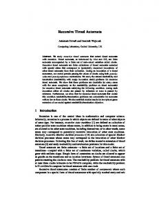
Object 2 occKind = periodic (period = (1,s) jitter = (10,ms)
msgSize = (64, bytes) deadline = (31.25, us)
Msg 2 () Msg 1() execTime = (6, ms) blockingTime = (8, ms) Action()
(t ≤ 3)
dx dt
Fig. 6.
Object 1
Fig. 7. UML Sequence Diagram annotated with MARTE stereotypes..
S0
S1
> Scenario
S2
Probabilistic Hybrid Automaton example.
Pros: PHyA (i) allow modeling non-determinism and (ii) allow for the modeling of continuous variables. Cons: PHyA (i) work with multiple clocks, (ii) support only flat structures, (iii) allow state invariants, and (iv) can not be verified formally in the general case. H. Unified Modeling Language (UML) and MARTE profile Apart from the above mentioned formalisms, one of the well known formalism for modeling industrial automation systems is ‘Unified Modeling Language’ (UML). UML was accepted as a standard by Object Management Group (OMG) in November 1997 [20]. Over the years several versions of UML have evolved; the latest adopted version is UML 2.2 [21]. UML statecharts can be defined as a 8 tuple A = (S, S0 , F, Σ, E, G, SH, DH), where S is a finite set of states, S0 ∈ S is the initial state, F ⊆ S is a distinguished set of final states/ accepted states, Σ is a finite set of triggers or input alphabets, E ⊆ S ×Σ×S ×Act is a set of transition functions of A - where Act defines the actions to be performed during the transition, G is the guard of the transition and the pseudo states: shallow and deep history are specified by SH and DH respectively. The recently standardized UML profile for Modeling and Analysis of Real-Time and Embedded systems (MARTE) [22] helps overcome the abstraction of time and time related concepts made by the basic metamodel of UML. UML MARTE introduces domain specific ideas relevant for modeling realtime embedded systems, involving the ability to express nonfunctional properties, execution platforms, quantifiable notions of time, etc. available within the UML framework. Figure 7 shows an UML diagram annotated with MARTE stereotypes.
The architecture of MARTE profile consists of three main packages namely the ‘MARTE Foundation package’, which defines all the basic foundational concepts required for the design and analysis of real-time and embedded systems, then the ‘MARTE Design Model’, which addresses model-based design starting from requirement capture to specification, design and implementation, and finally, the ‘MARTE Analysis Model’, which offers specific abstractions and relevant annotations that could be read by analysis tools. MARTE analysis is intended to provide trustworthy evaluations using formal quantitative analysis based on mathematical models. The GQAM subpackage aids model designers to specify details for generic quantitative analysis. The other two sub-packages mainly deal with schedulability (SAM) and performance analysis (PAM). III. C ONCLUSION In this paper, we provide a broad overview of the huge set of timed automata formalisms that exist in the field of system analysis and engineering. Comparison of the formalisms revealed their diverse nature and potential (refer table I). Every timed automata formalism has its pros and limitations as discussed in section II. Hence, model developers should be careful while identifying the appropriate formalism for their task; for e.g. some of the formalisms discussed in this paper are very well suited for describing/ modeling complex real-time systems; however, when it comes to building statistical models, these formalisms lack simplicity (i.e. several research works [23], [1], [24] show that the complexity of the verification problem of timed automata is exponential on the number of clocks used in the model — most of the formalisms discussed in this paper support multiple clocks; thus posing an important obstacle to the development of verification algorithms which are efficient in practice). Hence, for our future task of building statistical models from timed automata, we strongly feel the need for a simple but still a powerful formalism for building statistical models. R EFERENCES [1] R. Alur and D. Dill, “A theory of timed automata,” Theoretical Computer Science, vol. vol. 126, pp. 183–235, 1994. [2] A. David and M. O. M¨oller, “From huppaal to uppaal: A translation from hierarchical timed automata toflat timed automata,” BRICS, BRICS Report Series RS-01-11, Tech. Rep., March 2001.
[3] S. Burmester, “Generierung von java real-time code f¨ur zeitbehaftete uml modelle,” Master’s thesis, University of Paderborn, Department of Computer Science, Paderborn, Germany, September 2002. [4] H. Giese and S. Burmester, “Real-time statechart semantics,” Lehrstuhl f¨ur Softwaretechnik, Universit¨at Paderborn, Paderborn, Germany, Tech. Rep. tr-ri-03-239, June 2003. [5] M. Gehrke, P. Nawratil, O. Niggemann, and W. S. M. Hirsch, “Scenario-based verification of automotive software systems,” in Proc. of the Dagstuhl-Workshop: Model-Based Development of Embedded Systems(MBEES), 9.-13.1.2005, Schloss Dagstuhl, Germany, H. Giese, B. Rumpe, and B. Sch¨atz, Eds., 2006, pp. 35–42. [6] C. Dima, “Real-time automata,” Journal of Automata, Languages and Combinatorics, vol. Vol. 6, Issue 1, pp. 3 – 23, January 2001. [7] S. Verwer, M. de Weerdt, and C. Witteveen, “An algorithm for learning real-time automata,” in Proc. of the Sixteenth Annual Machine Learning Conference of Belgium andthe Netherlands (Benelearn), M. van Someren, S. Katrenko, and P. Adriaans, Eds., 2007, pp. 128–135. [8] M. Kwiatkowska, G. Norman, R. Segala, and J. Sproston, “Automatic verification of real-time systems with discrete probability distributions,” Theoretical Computer Science, vol. 282, pp. 101–150, 2002. [9] R. Alur, C. Courcoubetis, N. Halbwachs, T. A. Henzinger, P. h. Ho, X. Nicollin, A. Olivero, J. Sifakis, and S. Yovine, “The algorithmic analysis of hybrid systems,” Theoretical Computer Science, vol. 138, pp. 3–34, 1995. [10] J. Sproston, “Decidable model checking of probabilistic hybrid automata,” in FTRTFT, 2000, pp. 31–45. [11] J. S. Dong, P. Hao, and et.al, “Timed automata patterns,” IEEE Transactions on Software Engineering, vol. Vol 34, no. No. 6, December 2008. [12] A. David and W. Yi, “Hierarchical timed automata,” 2000, contacts:
[email protected],
[email protected]. [13] H. Giese, M. Tichy, S. Burmester, W. Sch¨afer, and S. Flake, “Towards the compositional verification of real-time uml designs,” in Proc. of the 9th European software engineering conference held jointly with 11th ACM SIGSOFT international symposium on Foundations of software engineering (ESEC/FSE-11). ACM Press, September 2003, pp. 38–47. [14] S. Burmester and H. Giese, “The fujaba real-time statechart plugin,” in Proc. of the first International Fujaba Days 2003, Kassel, Germany, H. Giese and A. Z¨undorf, Eds. University of Paderborn, October 2003, pp. 1–8. [15] S. Burmester, H. Giese, M. Hirsch, D. Schilling, and M. Tichy, “The fujaba real-time tool suite: Model-driven development of safety-critical, real-time systems,” in Proc. of the 27th International Conference on Software Engineering (ICSE), St. Louis, Missouri, USA. ACM Press, May 2005, pp. 670–671. [16] B. Kumar and J. Jasperneite, “Industrial communication protocol engineering using uml 2.0: a case study,” in 7th International Workshop on Factory Communication Systems (WFCS 2008), Dresden, Germany, May 2008. [17] B. Kumar, J. Imtiaz, and J. Jasperneite, “Applicability of uml marte’s schedulability sub-package for engineering industrial real-time protocols,” in 2nd Junior Researcher Workshop on Real-Time Computing (JRWRTC 2008) (in conjunction with the 16th International Conference on Real-Time and Network Systems (RTNS 2008)), Rennes, France, Oct 2008. [18] J. R. Norris, Markov Chains. Cambridge University Press, 1997. [19] P. Bremaud, Markov Chains - Gibbs Fields, Monte Carlo Simulation, and Queues. Springer Verlag, 1999. [20] OMG, OMG Unified Modeling Language Specification, Version 1.1, OMG, 1998. [21] ——, OMG Unified Modeling Language, Superstructure, Version 2.2, omg document number: formal/2009-02-02 ed., OMG, February 2009. [22] ——, A UML Profile for MARTE, OMG Adopted Specification, Version Beta 1, omg document number: ptc/07-08-04 ed., OMG, August 2007. [23] R. Alur, C. Courcoubetis, and D. Dill, “Model-checking in dense realtime,” Information and Computation, vol. 104, pp. 2–34, 1993. [24] C. Daws and S. Yovine, “Reducing the number of clock variables of timed automata,” in RTSS ’96: Proceedings of the 17th IEEE Real-Time Systems Symposium. Washington, DC, USA: IEEE Computer Society, 1996, pp. 73–81.