custom type class for totally ordered dense abelian groups, we worked on the concrete type ... and r :: c list is a list
Formalized Timed Automata Simon Wimmer? Institut f¨ ur Informatik, Technische Universit¨ at M¨ unchen
Abstract. Timed automata are a widely used formalism for modeling real-time systems, which is employed in a class of successful model checkers such as UPPAAL. These tools can be understood as trust-multipliers: we trust their correctness to deduce trust in the safety of systems checked by these tools. However, mistakes have previously been made. This particularly regards an approximation operation, which is used by modelchecking algorithms to obtain a finite search space. The use of this operation left a soundness problem in the tools employing it, which was only discovered years after the first model checkers were devised. This work aims to provide certainty to our knowledge of the basic theory via formalization in Isabelle/HOL: we define the main concepts, formalize the classic decidability result for the language emptiness problem, prove correctness of the basic forward analysis operations, and finally outline how both streams of work can be combined to show that forward analysis with the common approximation operation correctly decides emptiness for the class of diagonal-free timed automata.
1
Introduction
The foundations of the theory of timed automata are presented in the seminal work of Alur and Dill [1, 2]. They introduced the formalism as a model for systems with real-time constraints and showed how to decide the language emptiness problem via the so-called region construction. Unfortunately, the number of regions explored by this algorithm is exponential in the size of the automaton under consideration. Moreover, Alur and Dill also showed that the language emptiness problem for timed automata is PSPACE-hard. Still, the formalism is employed in practical model checking [12, 13, 19] by means of algorithms based on Difference Bound Matrices (DBMs). These algorithms (with some more elaborate optimizations) can cope with many interesting real-life model checking problems. The search space examined by the DBM algorithms is potentially infinite. Therefore an approximation is used to obtain a finite search space. The basic idea is to represent every state (called zone) by the smallest set of regions which contains the state. ?
Supported by DFG project NI 491/16-1
It took nearly a decade after this operation was initially devised, until Patricia Bouyer discovered [5] that the common algorithmic realization of this operation diverges from its intended result: the computed result is always a convex union of regions, whereas the smallest set of regions containing a zone can be non-convex. This left a soundness problem, which fortunately vanishes for the restricted class of so-called diagonal-free timed automata [6] (Section 2.1 precisely characterizes this class). While not as expressive as the full formalism of timed automata, this class is sufficient for modeling most of the problems of practical interest, which explains why the problem was not discovered for many years. This work aims to solidify the theoretical grounds on which real-time model checking with diagonal-free timed automata stands, by formalizing the basic theory and algorithms in Isabelle/HOL, and then going the full length to prove Bouyer’s correctness result. Section 2 will present the formalization of the basic notions for diagonal-free timed automata. Then Section 3 will show how we formalized DBMs and obtained soundness and completeness results for their basic algorithms. This includes a formalization of the Floyd-Warshall algorithm. Afterwards (Section 4) we define the notion of regions and prove that they are suitable for deciding the emptiness problem on timed automata. Finally, in Section 5, a refined version of these regions will be used to precisely formalize the approximation operation. To tie the ends of our formalization together, this characterization of approximation will be connected with its algorithmic version. This enables us to reuse the decidability result on the first region construction to prove that DBM-based algorithms together with approximation can decide the language emptiness problem for diagonal-free timed automata. For lack of space, many of our definitions and proofs are shortened or stated informally. We refer the reader to the entry in the Archive of Formal Proofs [15] for the full version (over 18500 lines). 1.1
History and Related Work
As mentioned, the basic theory was devised by Alur and Dill [1, 2]. The use of DBMs was also proposed by Dill [10] and brought to practical model checking by Yi et al. [18]. Bouyer’s developments of our main correctness results are spread over two papers. The first one presents a generalization of timed automata to updatable timed automata and revisits the basic decidability results for this class [7]. The second one [6] connects these results with DBMs to prove that the combination of DBM-based forward analysis operations and approximation decides the language emptiness problem. We are aware of one previous proof-assistant formalization of timed automata using PVS [16, 17]. This work has the basic decidability result using regions and claims to make some attempt to extend the formalization towards DBMs. Another line of work [11, 14] aims at modeling the class of p-automata [3] (which is undecidable in the general case) in Coq and proving properties of concrete p-automata within Coq. A similar approach was pursued with the help of Isabelle/HOL in the CClair project [8]. In contrast, the most important contributions of our work are the full formalization of the relevant DBM algorithms,
and particularly the rather intricate developments towards the correctness proof for the approximation operation – both of which pertain to practical real-time model checking. Unless otherwise stated, our formalizations of the basic notions and DBMs are based on a popular tutorial by Bengtsson and Yi [4], while the developments for the region constructions and the final correctness result follow Bouyer’s precise work.
2 2.1
Diagonal-Free Timed Automata in Isabelle/HOL Syntactic Definition
Compared to standard finite automata, timed automata introduce a notion of clocks. We will fix a type 0c for the space of clocks, type 0t for time, and a type 0 s for locations. While most of our formalizations only require 0t to belong to a custom type class for totally ordered dense abelian groups, we worked on the concrete type real for the region construction for simplicity. Fig. 1 depicts an example of a diagonal-free timed automaton. c1 ≤ 3, a1 , c1 := 0 c1 < 1, a2 , c2 := 0 s1
s2
c1 ≤ 3
c1 > 2 ∧ c2 ≤ 2 a3
Fig. 1: Example of a diagonal-free timed automaton with two clocks.
Locations and transitions are guarded with clock constraints, which have to be fulfilled to stay in a location or to transition between them. The variants of these constraints are modeled by datatype ( 0c, 0t) cconstraint = AND (( 0c, 0t) cconstraint) (( 0c, 0t) cconstraint) | LT 0c 0t | LE 0c 0t | EQ 0c 0t | GT 0c 0t | GE 0c 0t where the atomic constraints in the second line represent the constraint c ∼ d for ∼ = , ≥, respectively. The sole difference to the full class of timed automata is that those would also allow constraints of the form c 1 − c 2 ∼ d. We define a timed automaton A as a pair (T , I) where I :: 0s ⇒ ( 0c, 0t) cconstraint is an assignment of clock invariants to locations; T is a set of transitions written as A ` l −→g,a,r l 0 where – l :: 0s and l 0 :: 0s are start and successor location,
– g :: ( 0c, 0t) cconstraint is the guard of the transition, – a :: 0a is an action label, – and r :: 0c list is a list of clocks that will be reset to zero when the transition is taken. Standard definitions of timed automata would include a fixed set of locations with a designated start location and a set of end locations. The language emptiness problem usually asks if any number of legal transitions can be taken to reach an end location from the start location. Thus we can confine ourselves to study reachability and implicitly assume the set of locations to be given by the transitions of the automaton. Note that although the definition of clock constraints allows constants from the whole time space, we will later crucially restrict them to the natural numbers in order to obtain decidability.
2.2
Operational Semantics
We want to define an operational semantics for timed automata via an inductive relation. States of timed automata are pairs of a location and a clock valuation of type 0c ⇒ 0t assigning time values to clocks. Time lapse is modeled by shifting a clock valuation u by a constant value d : u ⊕ d = (λx . u x + d ). Finally, we connect clock valuations and constraints by writing, for instance, u ` AND (LT c 1 1 ) (EQ c 2 2 ) if u c 1 < 1 and u c 2 = 2. The precise definition is standard. Using these definitions, the operational semantics can be defined as a relation between pairs of locations and clock valuations. More specifically, we define action steps A ` l −→g,a,r l 0 ∧ u ` g ∧ u 0 ` inv-of A l 0 ∧ u 0 = [r →0 ]u A ` hl , ui →a hl 0, u 0i u ` inv-of A l ∧ u ⊕ d ` inv-of A l ∧ 0 ≤ d
. Here inv-of A ` hl , ui →d hl , u ⊕ d i (T , I) = I and the notation [r → 0 ]u means that we update the clocks in r to 0 in u. We write A ` hl , ui → hl 0,u 0i if either A ` hl , ui →a hl 0, u 0i or A ` hl , ui →d hl 0, u 0i. and delay steps via
2.3
Zone Semantics
The first conceptual step to get from this abstract operational semantics towards concrete algorithms on DBMs is to consider zones. Informally, the concept is simple; a zone is the set of clock valuations fulfilling a clock constraint: ( 0c, 0t) zone ≡ ( 0c ⇒ 0t) set. This allows us to abstract from a concrete state hl , ui to a pair of location and zone hl , Z i. We need the following operations on zones: Z ↑ = {u ⊕ d | u ∈ Z ∧ 0 ≤ d } and Z r → 0 = {[r →0 ]u | u ∈ Z }.
Naturally, we define a zone-based semantics by means of another inductive relation: A ` hl , Z i A ` hl , Z i
hl , (Z ∩ {u | u ` inv-of A l })↑ ∩ {u | u ` inv-of A l }i A ` l −→g,a,r l 0 hl 0, (Z ∩ {u | u ` g})r → 0 ∩ {u | u ` inv-of A l 0}i
With the help of two easy inductive arguments one can show soundness and completeness of this semantics w.r.t. the original semantics (where ∗ is the Kleene star operator): (Sound) A ` hl , Z i ∗ hl 0, Z 0i ∧ u 0 ∈ Z 0 =⇒ ∃ u∈Z . A ` hl , ui →∗ hl 0, u 0i (Complete) A ` hl , ui →∗ hl 0, u 0i ∧ u ∈ Z =⇒ ∃ Z 0. A ` hl , Z i ∗ hl 0, Z 0i ∧ u 0 ∈ Z 0 This is an example of where proof assistants really shine. Not only are our Isabelle proofs shorter to write down than for example the proof given in [18] – we have also found that the less general version given there (i.e. where Z = {u}) yields an induction hypothesis that is not strong enough in the completeness proof. This slight lapse is hard to detect in a human-written proof.
3 3.1
Difference Bound Matrices Fundamentals
Difference Bound Matrices constrain differences of clocks (or more precisely, the difference of values assigned to individual clocks by a valuation). The possible constraints are given by: datatype 0t DBMEntry = Le 0t | Lt 0t | ∞ This yields a simple definition of DBMs: 0t DBM ≡ nat ⇒ nat ⇒ 0t DBMEntry. To relate clocks with rows and columns of a DBM, we use a numbering v :: 0 c ⇒ nat for clocks. DBMs will regularly be accompanied by a natural number n, which designates the number of clocks constrained by the matrix. Although this definition complicates our formalization at times, we hope that it allows us to easily obtain executable code for DBMs while retaining a flexible “interface” for applications. To be able to represent the full set of clock constraints with DBMs, we add an imaginary clock 0, which shall be assigned to 0 in every valuation. Zero column and row will always be reserved for 0 (i.e. ∀ c. v c > 0 ). If necessary, we assume that v is an injection or surjection for indices less or equal to n. Informally, the zone [M ]v ,n represented by a DBM M is defined as {u | ∀ c 1 , c 2 , d . v c 1 , v c 2 ≤ n −→ (M (v c 1 ) (v c 2 ) = Lt d −→ u c 1 − u c 2 < d ) ∧ (M (v c 1 ) (v c 2 ) = Le d −→ u c 1 − u c 2 ≤ d )}
assuming that v 0 = 0. Example 1. 0 0 ∞ Lt c1 ∞ c 2 Le 4
c1 c2 ! (−3 ) Le 0 ∞ ∞ ∞ ∞
0 c1 c2 ! 0 Le 0 Lt (−3 ) Le 0 c1 ∞ Le 0 ∞ c 2 Le 4 Lt 1 Le 0
0 c1 c2 ! 0 ∞ Le 0 Le 0 c 1 ∞ ∞ Lt (−3 ) c 2 ∞ Le 3 Le 0
The left two DBMs both represent the zone described by the constraint c 1 > 3 ∧ c 2 ≤ 4, while the DBM on the right represents the empty zone. 1 To simplify the subsequent discussion, we will set 0c = nat, v = id and assume that the set of clocks of the automaton in question is {1 ..n}. We define an ordering relation ≺ on 0t DBMEntry by means of a