Aug 23, 2009 - We also give a heuristic variant of the algorithm which is faster but ... also that the parametric max flow-min cut (a.k.a. graph-cut) was used in.
A Total Variation-based Graph Clustering Algorithm for Cheeger Ratio Cuts Xavier Bresson∗
Arthur Szlam
August 23, 2009
Abstract In this work, inspired by [3] and [13], we give a continuous relaxation of the Cheeger cut problem on a weighted graph. We show that the relaxation is actually equivalent to the original problem, and based on [8, 16], we give an algorithm which experimentally is very efficient on some clustering benchmarks. We also give a heuristic variant of the algorithm which is faster but often gives just as accurate clustering results.
1
Introduction
Over the past several years, spectral clustering methods have become very popular; see [12] and [14] for an excellent introduction. These methods start with a (nonnegative, symmetric) matrix W which collects the relative similarities between a set of points V to be clustered, and then makes the assumption that in some sense, the cluster indicators should be smooth with respect to W . A simple such notion is that the length of the boundary of the clusters should be small relative to their area. This motivates the definition of the Cheeger cut value of a partition P = {V1 , V2 } of V into two pieces given by C(V1 , V2 ) =
Cut(V1 , V2 ) , min(|V1 |, |V2 |)
where
X
Cut(V1 , V2 ) =
Wij ,
i∈V1 ,j∈V2
and |V | is just the cardinality of V . Since finding the optimal Cheeger cut is NP-hard, the Cheeger cut is usually approximated by thePsecond eigenvalue of the combinatorial Laplacian D − W , where Dii = j Wij , such that: 1 C 2 ≤ λ2 ≤ 2C. 2 maxi Dii ∗ Authors are with the Department of Mathematics, University of California, Los Angeles, USA. Email: {aszlam,xbresson}@math.ucla.edu. This work was supported in part by ONR N00014-03-1-0071 and ONR MURI subcontract from Stanford University.
1
See [4] for the continuous version, and for the discrete version, see [5]. Note also that the parametric max flow-min cut (a.k.a. graph-cut) was used in 1 ,V2 ) [9] to minimize the biased ratio cut Cut(V , but cannot be used to solve |V1 | 1 ,V2 ) the unbiased ratio cut defined as Rcut(V1 , V2 ) = Cut(V + |V1 | which is NP-hard. Using the Raleigh quotient formula for the eigenvalue gives
λ2 = arg
Cut(V1 ,V2 ) , |V2 |
min H2 (f )
f ∈L2 (V )
P
= arg
min
f ∈L2 (V
)
||∇f ||2 , ||f − M (f )||22
where for p ≥ 1, ||∇f ||p at i is given by X ||∇f ||p (i) = Wij |f (i) − f (j)|p , j
and where M (f ) is the mean of f . The functional H2 measures smoothness. It has long been known that L2 measures of smoothness are not as well suited for dealing with functions with jumps as L1 measures of smoothness; in image processing, see for example [11]. Very recently in [3] (also see [1]), it was shown that P p i ||∇f || (i) lim min p = min C(P ). p7→1 f minc ||f − c||p P With this in mind we can relax the problem min C(P ) P
as follows: for any binary valued function f = χV1 , V1 ( V , ½ |V2 | |V1 | > |V2 | ||f − m(f )||1 = |V1 | |V1 | ≤ |V2 |, where m(f ) is the median of f , and V2 is the compliment in V of V1 . Then P P P vi ∈V1 vj ∈V2 Wij i ||∇fP ||(i) =2 ||fP − m(fP )||1 min(|V1 |, |V2 |) = 2C(V1 , V2 ). Thus
P
i ||∇f ||(i) ||f − m(f )||1 is a relaxation of the Cheeger cut problem, and P i ||∇f ||(i) min ≤ min C(P ). P f ||f − m(f )||1
min f
(1)
In this work we will show that the inequality (1) is actually an equality, and for any solution f of the relaxed minimization that there is a threshold γ so that the binary function ½ 1 f >γ fγ = 0 f ≤ γ,
2
has the same energy as the minimum cut. A similar approach has been studied in the continuous setting by Strang in [13]. We will then give an algorithm for minimizing the ratio energy which is experimentally efficient, and then another algorithm for minimizing a similiar but easier energy. Finally, we will provide some experiments on the quality of the clusterings given by the algorithms we have presented.
2 Equivalence of the TV problem and the Ratio Cut problem In this section we fix a set of points V and a similarity matrix W between these points. For a function f : V 7→ R X |f |TV = ||∇f ||. i
Note that this is a norm on the set of function modulo constants. As before, denote the median of f by m(f ). Lemma 2.1. A function f : V 7→ R is an extreme point of the TV unit ball if and only if there is a number α such that f = αχS , where S ( V . Proof. Denote by {a1 , ..., an } the distinct values of f arranged in increasing order. Let Sr = {v : f (v) = ar }, Sr+ = {v : f (v) > ar }, and Sr− = {v : f (v) < ar } pick indices t and s with t 6= s, and let g = f + ²s χSs + ²t χSt ; and h = f − ²s χSs − ²t χSt , where ²s and ²t will be chosen in a moment. Note that adding ²s χSs to f changes its total variation by X X ²s Wij − Wij , − i∈Ss ,j∈Ss
+ i∈Ss ,j∈Ss
and adding ²t χSt to the resulting function changes the total variation by the corresponding expression with St , and and as long as ²s and ²t are chosen small enough to not upset the order of the values of f , the changes are independent. Thus by keeping P P + Wij − Wij − i∈S ,j∈Ss Pi∈Ss ,j∈Ss ²s = − P s ²t , Wij − i∈St ,j∈S + Wij i∈St ,j∈S − t
t
and picking both small enough so that the order of the values does not change, we get that |g|TV = |h|TV = 1. Then f = g/2 + h/2, and so f is not an extreme point of the ball. To prove the converse, let f = αχS , and suppose that βg + (1 − β)h = f , for some g and h in the TV unit ball on W . Let W ∗ be the weighted subgraph of W given by ½ Wij i ∈ S and j ∈ S c ∗ Wij := 0 otherwise, Note that on W ∗ , still βg + (1 − β)h = f ; and |f |TV(W ∗ ) = 1. By the sublinearity of the TV(W ∗ ) norm 1 ≤ β|g|TV(W ∗ ) + (1 − β)|h|TV(W ∗ ) ,
3
but the choice of g and h show that β|g|TV(W ∗ ) + (1 − β)|h|TV(W ∗ ) ≤ β + (1 − β) = 1, and so 1 = |g|TV(W ∗ ) and |h|TV(W ∗ ) = 1. Therefore both h and g are constant on S and S c , and were thus, up to a constant, multiples of f . We will need a slightly sharper version of of Lemma 2.1 below; however, the proof is essentially the same. Lemma 2.2. Let W be a weighted graph, and let I+ and I− be a partition of V . Let Q be the set of vectors in Rn such that f is nonnegative in the coordinates I+ , and nonpositive in the coordinates I− ; let B be the TV norm unit ball on Q. The vector f is an extreme points of B if and only if there exists a number α with f = αχS , where S ( V . Proof. The “if” direction is as above. The proof of the “only if” direction proceeds exactly as in Lemma 2.1 if f takes positive and negative values. If f takes nonegative values, then the proof above works as long as we choose at > as > 0; and similarly for the nonpositive case. Theorem 2.3. Consider the problem λ = min f
|f |TV . ||f − m(f )||1
There is a binary valued minimizer, and λ = min S
Cut(S) . min (|S|, |S c |)
Furthermore, for any minimizer f , there is a number γ so that the function ½ 1 f >γ fγ = 0 f ≤ γ, is also a minimizer. Proof. Suppose f is a minimizer. If |f |TV = 0, the characteristic function of the support of f is binary and also has TV norm zero. If not, because the functional has homogeneity 0, we can rescale f to fix the numerator of the energy as |f |TV = 1; f is thus a maximizer for the denominator, constrained to the TV ball. Because both numerator and denominator are unchanged by the addition of a constant to f , we may restrict attention to f with m(f ) = 0. Let I1 be the indices where f ≤ 0, and let I2 be the indices where f > 0. Note that any function nonpositive on I1 and nonnegative on I2 also has median 0; denote this set of functions by Q. Denote by B the TV norm unit ball on Q. By definition, f is a solution to maxB ||f ||1 . The set B is convex, and || · ||1 is a convex function on B, so it takes its maximum at an extreme point; by Lemma 2.2, there is a
4
binary valued maximizer g = αχS for some set S, and the energy of g is Cut(S) exactly min(|S|,|S c |) . To see the last part of the statement, note that f can be written as P f = βi gi where the giP are extreme points (and therefore characteristic functions), βi > 0, and βi = 1. Because the L1 norm is linear on the quadrant that f lies in, all the gi are also minimizers. It thus suffices to pick γ to be the value of the greatest valued gi .
3 A Split-Bregman algorithm for ratio minimization In this section, we show how to solve two minimization problems. The first minimzation problem is the following: min f ∈R
|f |TV ||f − m(f )||1
which is equivalent to solve the constrained minimization problem [6]: min max |f |TV − λ||f ||1 s.t. m(f ) = 0. u
λ
We will use the following iterative process: Algorithm 1: While not converged do: 1. f n+1/2 = arg minf |f |TV − λn ||f ||1 (*) 2. f n+1 = f n+1/2 − m(f n+1/2 ) 3. λn+1 = |f n+1 |TV /||f n+1 ||1 End while. The minimization problem (*) belongs to the class of L1-regularized problems. Several schemes have been introduced in the literature to solve this class of problems. In this work, we will use the efficient split-Bregman method originally introduced in [8] to solve the TVL2 problem and the compressed sensing problem and extended in [16] for the non-local/graph framework. However, the minimization (*) is slightly different from [8, 16] for two reasons. Firstly, it uses a negative L1 term, i.e. −||f ||1 , which requires a new minimizing operator different from wavelet shrinkage. Secondly, the graph-based TV norm is anisotropic unlike the anisotropic graph-based TV defined in [16]. We now develop the numerical scheme. Energy (*) can be written as: XX wij |fj − fi | − λ|fi |. min f
i
j∼i
We introduce two splitting variables to deal with the two L1 norms: XX min wij |dij | − λ|ei | s.t. dij = fj − fi , ei = fi . f,d,e
i
j∼i
5
Then, the Bregman iteration method [2, 10] is used to solve the previous constrained minimization problem as follows: P P (f k+1 , dk+1 , ek+1 ) = arg minf,d,e i j∼i wij |dij | − λ|ei |+ λ1 (dij − (fj − fi ) − bkij )2 + λ22 (ei − fi − cki )2 2 bk+1 = bkij + fjk+1 − fik+1 − dk+1 ij ij k+1 ei = eki + fik+1 − ek+1 i
(2)
The first line is solved by alternate minimization since the total energy is convex. First, the Euler-Lagrange equation of the minimization problem w.r.t. f defined as: min f
X X λ1 λ2 (dij − (fj − fi ) − bkij )2 + (ei − fi − cki )2 2 2 i j∼i
is given by: X λ1 (dij − dji − 2(fj − fi ) − bkij + bkji ) + λ2 (fi − ei + cki ) = 0 j∼i
whose solution, we call f k+1 , is given by a few Gauss-Seidel iterations as follows: ³ ´ X 1 P − λ1 (dij − dji − bkij − 2fjm + bkji ) + λ2 (ei − cki ) (3) fik+1,m+1 = 2λ1 j∼i +λ2 j∼i starting from f k+1,m=0 = f k . The minimization process (2) w.r.t. d is defined as: min d
XX i
wij |dij | +
j∼i
λ1 (dij − (fjk+1 − fik+1 ) − bkij )2 2
whose solution is known as the shrinkage operator [7]: dk+1 = ij
³ wij ´ k+1 k+1 k ,0 max |f − f + b | − ij j i λ1 |fjk+1 − fik+1 + bkij | fjk+1 − fik+1 + bkij
(4)
Finally, the minimization process (2) w.r.t. e is: min e
X i
−λ|ei | +
λ2 (ei − ui − cki )2 2
(5)
whose solution is different from the minimizing solution given by the shrinkage operator as in (4) because of the minus sign in front of the L1 norm, i.e. −|.|. However, the minimizing solution of (5) has also a nice closed-form solution defined as: ek+1 = fik+1 + cki + i
fik+1 + cki λ |fik+1 + cki | λ2
(6)
Alternating (3), (4) and (6) until convergence provides the solution f n+1/2 = f k→∞ .
6
The second minimization problem that we want to solve is the following (this iterative scheme is faster than the previous one): Algorithm 2: While not converged do: 1. Minimize a few steps |f |TV , call f n+1/3 the solution after a few steps (**) 2. f n+1/2 = f n+1/3 − mean(f n+1/3 ) P n+1/2 3. Compute f n+1 s.t. = ct i fi End while. The minimization step (**) can be done using a similar approach as the first model. Indeed, a few steps of minimization of (**) can be done with this iterative scheme: P P ½ λ1 k 2 (f k+1 , dk+1 ) = arg minf,d,e i j∼i wij |dij | + 2 (dij − (fj − fi ) − bij ) k+1 k+1 k+1 k+1 k bij = bij + fj − fi − dij The minimization w.r.t. f is done by a few Gauss-Seidel iterations as follows: X 1 (dij − dji − 2fjm − bkij + bkji ) fik+1,m+1 = − P 2 j∼i j∼i starting from f k+1,m=0 = f k . Finally, the minimizing solution w.r.t. d is: dk+1 = ij
4
fjk+1 − fik+1 + bkij |fjk+1
−
fik+1
+
bkij |
³ wij ´ max |fjk+1 − fik+1 + bkij | − ,0 λ1
Experiments
In all experiments we use a 10-N N graph with the self-tuning weights as in [15], and the neighbor parameter set to 10. The optimization parameters for algorithm 1 for all expriments are fixed as follows: λ1 = 1, λ2 = 1.5, the number of n iterations is 15, the number of k iterations is 30 and the number of m is 5. The optimization parameters for algorithm 2 for all expriments are fixed as follows: λ1 = 0.3, the number of n iterations is 50, the number of k iterations is 1 and the number of m is 15. Both methods are intialized by multiplying the indicator of a random P point by the averaging-normalized weight matrix D−1 W (where Dii = j Wij ) 1000 times.
4.1
MNIST
We test on the combined training and test samples from the MNIST dataset, available at http://yann.lecun.com/exdb/mnist/. This data set consists of 70000 28 × 28 images of handwritten digits, 0 through 9. The data was preprocessed by projecting onto 50 principal components.
7
mode/true 0 1 1 2 3 4 6 7 8 9
0 6857 4 1 5 3 1 18 3 5 6
1 2 3642 4013 109 26 18 4 12 14 37
2 30 8 3 6855 15 4 5 34 30 6
3 3 3 4 48 6931 1 4 24 102 21
4 4 3 5 4 4 6612 15 10 6 161
5 26 1 0 1 6170 4 72 3 14 22
6 23 9 5 1 14 6 6815 0 3 0
7 3 13 10 36 5 20 0 7122 11 73
8 9 26 20 8 257 10 19 10 6448 18
Figure 1: Confusion matrix for the clustering of MNIST using the relaxed Cheeger model (Algorithm 1). Each row is a cluster; the number in the leftmost column of each row is the dominant label of that cluster. The 3’s and 5’s are merged, but otherwise the clustering is very accurate. The total computation time (not including constructing the weights) was 2710 seconds (∼ 45 minutes). The goal in this data set is to discover the 10 digit classes. The methods described above give a binary clustering, so in order to obtain 10 clusters, we iteratively subdivide in the standard way. That is, we tentatively divide each of the l current clusters in two, and keep the division minimizing the sum of the Cheeger cut values between each cluster and the union of all the others; now we have l + 1 clusters, and we repeat till we have 10. The confusion matrices for the results of the clustering using the relaxed Cheeger algorithm and the constrained TV algorithm are presented in Figures 1 and 4.1
4.2
Two moons
We construct the two moons data set as in [3]. We take the half of a circle of radius one in R2 with positive second coordinate sampled with a thousand points, and the half with negative second coordinate also sampled at a thousand points, but shifted 1 in the positive first coordinate direction, and .5 in the positive second coordinate direction. The data set is embedded in R100 , and Gaussian noise with σ = .02 is added. We calculate the clustering with the relaxed Cheeger cut model and the constrained TV model over 100 instantations of the data set. The average errors and run times are in Figure 4.2
8
9 12 1 5 5 170 56 3 62 33 6611
mode/true 0 1 1 2 3 4 6 7 8 9
0 6846 0 3 6 6 0 23 1 13 5
1 4 3983 3628 82 58 18 5 13 57 29
2 28 1 5 6834 20 5 6 54 30 7
3 2 0 2 46 6948 2 1 30 83 27
4 3 3 6 7 2 6598 49 9 5 142
5 17 0 1 1 6194 4 45 3 24 24
6 15 2 7 2 48 3 6786 0 13 0
7 7 10 17 30 5 23 0 7107 6 88
8 4 11 16 9 348 12 12 11 6379 23
Figure 2: Confusion matrix for the clustering of MNIST using the constrained TV model (Algorithm 2). Each row is a cluster; the number in the leftmost column of each row is the dominant label of that cluster. The 3’s and 5’s are merged, but otherwise the clustering is very accurate; the accuracy is only slightly less than the clustering using Algorithm 1. The total computation time (not including constructing the weights) was 428 seconds (∼ 7 minutes).
References [1] S. Amghibech. Eigenvalues of the discrete p-laplacian for graphs. Ars Comb., 67, 2003. [2] L. Bregman. The Relaxation Method of Finding the Common Points of Convex Sets and Its Application to the Solution of Problems in Convex Programming. USSR Computational Mathematics and Mathematical Physics, 7:200–217, 1967. [3] T. Buhler and M. Hein. Spectral Clustering based on the graph p-Laplacian. In International Conference on Machine Learning (ICML), 2009. [4] J Cheeger. A lower bound for the smallest eigenvalue of the laplacian. In RC Gunning, editor, Problems in Analysis, pages 195–199. Princeton Univ. Press. [5] F. R. K. Chung. Spectral graph theory, volume 92 of CBMS Regional Conference Series in Mathematics. Published for the Conference Board of the Mathematical Sciences, Washington, DC, 1997. [6] W. Dinkelbach. On Nonlinear Fractional Programming. Management Science, 13:492–498, 1967. [7] D. Donoho. De-Noising by Soft-Thresholding. IEEE Transactions on Information Theory, 41(33):613–627, 1995. [8] T. Goldstein and S. Osher. The Split Bregman Method for L1Regularized Problems. SIAM Journal on Imaging Sciences, 2(2):323– 343, 2009.
9
9 16 4 1 5 165 67 9 52 20 6619
(a) Second eigenvector of the Laplacian.
(b) Optimal Cheeger cut obtained by thresholding the second eigenvector of the Laplacian, value is 0.28.
(c) Output of algorithm 1.
(d) Optimal Cheeger cut obtained by thresholding the output of algorithm 1, value is 0.1.
10 (e) Histogram of the second eigenvector of the Laplacian.
(f) Histogram of the solution of the output of algorithm 1.
Figure 3: Results for the 4’s and 9’s in the MNIST dataset, 11791 points in 282 (= 784) dimensions.
|f |TV ||f − m(f P )||1 P |f |TV , f = 0, |f |=1 2nd Eigenvector method
8.2 13.8 16.4
Figure 4: Average error in percent on the two moons data set over 100 instances. |f |TV ||f − m(f )||1 |f P|TV , P f = 0, |f |=1 2nd Eigenvector method
5.6 .6 .05
Figure 5: Average runtime in seconds on the two moons data set over 100 instances, not counting time spent building the weights. [9] V. Kolmogorov, Y. Boykov, and C. Rother. Applications of Parametric Maxflow in Computer Vision. In International Conference on Computer Vision, pages 1–8, 2007. [10] S. Osher, M. Burger, D. Goldfarb, J. Xu, and W. Yin. An Iterative Regularization Method for Total Variation-based Image Restoration. SIAM Multiscale Modeling and Simulation, 4:460–489, 2005. [11] L. I. Rudin, S. Osher, and E. Fatemi. Nonlinear total variation based noise removal algorithms. Phys. D, 60(1-4):259–268, 1992. [12] J. Shi and J. Malik. Normalized cuts and image segmentation. IEEE Tran PAMI, 22(8):888–905, 2000. [13] G. Strang. Maximal Flow Through A Domain. Mathematical Programming, 26:123–143, 1983. [14] U. von Luxburg. A tutorial on spectral clustering. Technical Report 149, 08 2006. [15] L. Zelnik-Manor and P. Perona. Self-tuning spectral clustering. In Advances in Neural Information Processing Systems 17 (NIPS 2004), 2004. [16] X. Zhang, M. Burger, X. Bresson, and S. Osher. Bregmanized Nonlocal Regularization for Deconvolution and Sparse Reconstruction. CAM Report 09-03, 2009.
11
(a) Second eigenvector of the Laplacian.
(b) Optimal Cheeger cut obtained by thresholding the second eigenvector of the Laplacian, value is 0.60.
(c) Output of algorithm 1.
(d) Optimal Cheeger cut, value is 0.41.
(e) Histogram of the second eigenvector of the Laplacian.
(f) Histogram of the output of algorithm 1.
Figure 6: Results for the two moons dataset, 2000 points in 100 dimensions.
12