to extract domain-specific concepts from two different corpora and show that ..... Hypernym b fragilis, c albicans, l pneumophila, candida albicans, c albicans.
BorderFlow: A Local Graph Clustering Algorithm for Natural Language Processing Axel-Cyrille Ngonga Ngomo1 and Frank Schumacher1 Department of Business Information Systems University of Leipzig Johannisgasse 26, Leipzig D-04103, Germany {ngonga|schumacher}@informatik.uni-leipzig.de, WWW home page: http://bis.uni-leipzig.de/
Abstract. In this paper, we introduce BorderFlow, a novel local graph clustering algorithm, and its application to natural language processing problems. For this purpose, we first present a formal description of the algorithm. Then, we use BorderFlow to cluster large graphs and to extract concepts from word similarity graphs. The clustering of large graphs is carried out on graphs extracted from the Wikipedia Category Graph. The subsequent low-bias extraction of concepts is carried out on two data sets consisting of noisy and clean data. We show that BorderFlow efficiently computes clusters of high quality and purity. Therefore, BorderFlow can be integrated in several other natural language processing applications.
1
Introduction
Graph-theoretical models and algorithms have been successfully applied to natural language processing (NLP) tasks over the past years. Especially, graph clustering has been applied to areas as different as language separation [3], lexical acquisition [9] and word sense disambiguation [12]. The graphs generated in NLP are usually large. Therefore, most global graph clustering approaches fail when applied to NLP problems. Furthermore, certain applications (such as concept extraction) require algorithms able to generate a soft clustering. In this paper, we present a novel local graph clustering algorithm called BorderFlow, which is designed especially to compute a soft clustering of large graphs. We apply BorderFlow to two NLP-relevant tasks, i.e., clustering large graphs and concept extraction. We show that our algorithm can be effectively used to tackle these two tasks by providing quantitative and qualitative evaluations of our results. This paper is structured as follows: in the next section, we describe BorderFlow formally. Thereafter, we present our experiments and results. First, we present the results obtained using BorderFlow on three large similarity graphs extracted from the Wikipedia Category Graph (WCG). By these means, we show that BorderFlow can efficiently handle large graphs. Second, we use BorderFlow to extract domain-specific concepts from two different corpora and show that it computes concepts of high purity. Subsequently, we conclude by discussing possible extensions and applications of BorderFlow.
2
2
BorderFlow
BorderFlow is a general-purpose graph clustering algorithm. It uses solely local information for clustering and achieves a soft clustering of the input graph. The definition of cluster underlying BorderFlow was proposed by Flake et al. [5], who state that a cluster is a collection of nodes that have more links between them than links to the outside. When considering a graph as the description of a flow system, Flake et al.’s definition of a cluster implies that a cluster X can be understood as a set of nodes such that the flow within X is maximal while the flow from X to the outside is minimal. The idea behind BorderFlow is to maximize the flow from the border of each cluster to its inner nodes (i.e., the nodes within the cluster) while minimizing the flow from the cluster to the nodes outside of the cluster. In the following, we will specify BorderFlow for weighted directed graphs, as they encompass all other forms of non-complex graphs. 2.1
Formal Specification
Let G = (V, E, ω) be a weighted directed graph with a set of vertices V, a set of edges E and a weighing function ω, which assigns a positive weight to each edge e ∈ E. In the following, we will assume that non-existing edges are edges e such that ω(e) = 0. Before we describe BorderFlow, we need to define functions on sets of nodes. Let X ⊆ V be a set of nodes. We define the set i(X) of inner nodes of X as: i(X) = {x ∈ X|∀y ∈ V : ω(xy) > 0 → y ∈ X}.
(1)
The set b(X) of border nodes of X is then b(X) = {x ∈ X|∃y ∈ V \X : ω(xy) > 0}.
(2)
The set n(X) of direct neighbors of X is defined as n(X) = {y ∈ V \X |∃x ∈ X : ω(xy) > 0}.
(3)
In the example of a cluster depicted in Figure 2.1, X = {3, 4, 5, 6}, the set of border nodes of X is {3, 5} , {6, 4} its set of inner nodes and {1, 2} its set of direct neighbors. Let Ω be the function that assigns the total weight of the edges from a subset of V to another one to these subsets (i.e., the flow between the first and the second subset). Formally: Ω : 2VP× 2V → R Ω(X, Y ) = x∈X,y∈Y ω(xy). We define the border flow ratio F (X) of X ⊆ V as follows: � � Ω b(X), X Ω b(X), X �= �. F (X) = Ω b(X), V \X Ω b(X), n(X)
(4)
(5)
3
… 7
1
2 3 5
6 …
4 …
Fig. 1. An exemplary cluster. The nodes with relief are inner nodes, the grey nodes are border nodes and the white are outer nodes. The graph is undirected.
Based on the definition of a cluster by [5], we define a cluster X as a nodemaximal subset of V that maximizes the ratio F (X)1 , i.e.: ∀X 0 ⊆ V, ∀v ∈ / X : X 0 = X + v → F (X 0 ) < F (X).
(6)
The idea behind BorderFlow is to select elements from the border n(X) of a cluster X iteratively and insert them in X until the border flow ratio F (X) is maximized, i.e., until Equation (6) is satisfied. The selection of the nodes to insert in each iteration is carried out in two steps. In a first step, the set C(X) of candidates u ∈ V \X which maximize F (X + u) is computed as follows: C(X) := arg max F (X + u).
(7)
u∈n(X)
By carrying out this first selection step, we ensure that each candidate node u which produces a maximal flow to the inside of the cluster X and a minimal flow to the outside of X is selected. The flow from a node u ∈ C(X) can be divided into three distinct flows: – the flow Ω(u, X) to the inside of the cluster, – the flow Ω(u, n(X)) to the neighbors of the cluster and – the flow Ω(u, V \(X ∪ n(X))) to the rest of the graph. Prospective cluster members are elements of n(X). To ensure that the inner flow within the cluster is maximized in the future, a second selection step is necessary. During this second selection step, BorderFlow picks the candidates u ∈ C(X) which maximize the flow Ω(u, n(X)). The final set of candidates Cf (X) is then Cf (X) := arg max Ω(u, n(X)).
(8)
u∈C(X) 1
For the sake of brevity, we shall utilize the notation X + c to denote the addition of a single element c to a set X. Furthermore, singletons will be denoted by the element they contain, i.e., {v} ≡ v.
4
All elements of Cf (X) are then inserted in X if the condition F (X ∪ Cf (X)) ≥ F (X)
(9)
is satisfied. 2.2
Heuristics
One drawback of the method proposed above is that it demands the simulation of the inclusion of each node in n(X) in the cluster X before choosing the best ones. Such an implementation can be time-consuming as nodes in terminology graphs can have a high number of neighbors. The need is for a computationally less expensive criterion for selecting a nearly optimal node to optimize F (X). Let us assume that X is large enough. This assumption implies that the flow from the cluster boundary to the rest of the graph is altered insignificantly when adding a node to the cluster. Under this condition, the following two approximations hold: Ω(b(X), n(X)) ≈ Ω(b(X + v), n(X + v)), (10) Ω(b(X), v) − Ω(d(X, v), X + v) ≈ Ω(b(X), v). Consequently, the following approximation holds: ∆F (X, v) ≈
Ω(b(X), v) . Ω(b(X + v), n(X + v))
(11)
Under this assumption, one can show that the nodes that maximize F (X) maximize the following: f (X, v) =
Ω(b(X), v) for symmetrical graphs. Ω(v, V \X)
(12)
Now, BorderFlow can be implemented in a two-step greedy fashion by ordering all nodes v ∈ n(X) according to 1/f (X, v) (to avoid dividing by 0) and choosing the node v that minimizes 1/f (X, v). Using this heuristic, BorderFlow is easy to implement and fast to run.
3
Experiments and Results
In this section, we present two series of experiments carried out using BorderFlow. 3.1
Clustering Large Graphs
Experimental setup The global aim of this series of experiments was to generate a soft clustering of paradigmatically similar nodes from the WCG. The WCG2 is a directed cyclic 2
We used the version of July 2007
5
graph whose edges represent the is-a relation [15]. Therefore, we needed to define a similarity metric for the categories ζ of the WCG. We chose to use the Jaccard metric 2|R(ζ, r) ∩ R(ζ 0 , r)| σr (ζ, ζ 0 ) = (13) |R(ζ, r) ∪ R(ζ 0 , r)| on the sets R(x, r) = {y : r(x, y)}, (14) where r was one of the following three relations: – parent-of : parent-of (ζ, ζ 0 ) ⇔ ζ 0 is-a ζ. – child-of : child-of (ζ, ζ 0 ) ⇔ ζ is-a ζ 0 . – shared-article: shared-article(ζ, ζ 0 ) holds iff there exists a Wikipedia article that was tagged using both ζ and ζ 0 . To ensure that we did not generate polysemic clusters, we did not use hubs as seeds. In the context of our experiments, we defined hubs as nodes which displayed a connectivity above the average connectivity of the graph. In the graphs at hand, the average connectivity for parent-of was 295, 8 for child-of and 60 for shared-article. It is important to notice that nodes with a connectivity above average could be included in clusters. The quantitative evaluation of our clustering was carried out by using the silhouette index [11]. Results We tried clustering the three resulting similarity graphs using the MCL algorithm [14] but had to terminate the run after seven days without results. Table 1 sums up the results we obtained by using BorderFlow. There were 244,545 initial categories. The clustering based on child-of covered solely 31.63% of the categories available because a high percentage of the categories of the WCG do not have any descendant. The other two relations covered approximately the same percentage of categories (82.21% for shared-article and 82.07% for parent-of ). Table 1. Results on the WCG
Categories Coverage Clusters Average number of nodes per clusters Average number of clusters per node Mean silhouette Standard deviation
shared-article
child-of
parent-of
201,049 82.21% 93,331 3.59 7.74 0.92 0.09
77,292 31.61% 28,568 2.29 6.20 0.20 0.19
200,688 82.07% 90,418 8.63 19.15 0.74 0.24
Figure 2 shows the distribution of the silhouette over all the clusters computed on the three graphs. The best clustering was achieved on the sharedarticle-graph (see Figure 2(a)). We obtained the highest mean (0.92) with the
6
smallest standard deviation (0.09). An analysis of the silhouettes of the clusters computed by using the parent-of -graph revealed that the mean of the silhouette lied around 0.74 with a standard deviation of 0.24 (see Figure 2(b)). The smaller average silhouette value was mainly due to the high connectivity of the similarity graph generated using this relation, resulting into large clusters and thus a higher flow to the outside (see Table 1). Clustering the child-of -graph yielded the worst results, with a mean of 0.20 and a standard deviation of 0.19. Figure 3 shows an example of a cluster containing “Computational Linguistics”.
1 2 0 0
1 2 0 0
1 0 0 0
8 0 0
N u m b e r o f c lu s te r s
N u m b e r o f c lu s te r s
1 0 0 0
6 0 0
4 0 0
2 0 0
8 0 0
6 0 0
4 0 0
2 0 0
0 0
-1 ,0
-0 ,8
-0 ,6
-0 ,4
-0 ,2
0 ,0
0 ,2
0 ,4
0 ,6
0 ,8
1 ,0
-1 ,0
-0 ,8
-0 ,6
-0 ,4
S ilh o u e tte v a lu e s
-0 ,2
0 ,0
0 ,2
0 ,4
0 ,6
0 ,8
1 ,0
S ilh o u e tte v a lu e s
(a) Using shared-article
(b) Using child-of
2 5 0 0
N u m b e r o f c lu s te r s
2 0 0 0
1 5 0 0
1 0 0 0
5 0 0
0 -1 ,0
-0 ,8
-0 ,6
-0 ,4
-0 ,2
0 ,0
0 ,2
0 ,4
0 ,6
0 ,8
1 ,0
S ilh o u e tte v a lu e s
(c) Using parent-of Fig. 2. Distribution of silhouette values
The high average number of clusters per node (i.e., the number of cluster to which a given node belongs) show how polysemic the categories contained in the WCG are. By using the clustering resulting from our experiments with the shared-article relation, one can subdivide the WCG into domain-specific categories and use these to extract domain-specific corpora from Wikipedia. Furthermore, BorderFlow allows the rapid identification of categories similar to given seed categories. Thus, BorderFlow can be used for other NLP applications such as query expansion [2], topic extraction [8] and terminology expansion [7].
7
Fig. 3. An example of a cluster containing “Computational Linguistics”
3.2
Low-bias Concept Extraction
In our second series of experiments, we used BorderFlow for the low-bias extraction of concepts (i.e., semantic classes) from word similarity graphs. We were especially interested in providing a qualitative evaluation of the results of BorderFlow. For this purpose, we measured the purity of the clusters computed by BorderFlow against a reference data set. Experimental setup The input to our approach to concept extraction consisted exclusively of domainspecific corpora. Our approach was subdivided into two main steps. First, we extracted the domain-specific terminology from the input without using any apriori knowledge on the structure of the language to process or the domain to process. Then, we clustered this terminology to domain-specific concepts. The low-bias terminology extraction was carried out by using the approach described in [9] on graphs of the size 20,000. Our experiments were conducted on two data sets: the TREC corpus for filtering [10] and a subset of the articles published by BioMed Central (BMC3 ). Henceforth, we will call the second corpus BMC. The TREC corpus is a test collection composed of 233,445 abstracts of publications from the bio-medical domain. It contained 38,790,593 running word forms. The BMC corpus consists of full text publications extracted from the BMC Open Access library. The original documents were in XML. We extracted the text entries from the XML data using a SAX4 Parser. Therefore, it contained a large amount of impurities that were not captured by the XML-parser. The main idea behind the use of this corpus was to test our method on real life data. The 13,943 full text documents contained 70,464,269 running word forms. 3 4
http://www.biomedcentral.com SAX stands for Simple Application Programming Interface for XML.
8
For the extraction of concepts, we represented each of the domain-specific terms included in the terminology extracted priorly by its most significant cooccurrences [6]. These were computed in two steps. In a first step, we extracted function words by retrieving the f terms with the lowest information content according to Shannon’s law [13]. Function words were not considered as being significant co-occurrences. Then, the s best scoring co-occurrences of each term that were not function words were extracted and stored as its feature vector. The similarity values of the features vectors were computed by using the cosine metric. The resulting similarity values were used to compute a term similarity graph, which was utilized as input for BorderFlow. We evaluated our results quantitavely and qualitatively. In the quantitative evaluation, we compared the clustering generated by BorderFlow with that computed using kNN, which is the local algorithm commonly used for clustering tasks. In the qualitative evaluation, we computed the quality of the clusters extracted by using BorderFlow by comparing them with the controlled MEdical Subject Headings (MESH5 ) vocabulary. Quantitative evaluation In this section of the evaluation, we compared the average silhouettes [11] of the clusters computed by BorderFlow with those computed by kNN on the same graphs. To ensure that all clusters had the same maximal size k, we used the following greedy approach for each seed: first, we initiated the cluster X with the seed. Then, we sorted all v ∈ n(X) according to their flow to the inside of the cluster Ω(v, X) in the descending order. Thereafter, we sequentially added all v until the size of the cluster reached k. If it did not reached k after adding all neighbors, the procedure was iterated with X = X ∪ n(X) until the size k was reached or no more neighbors were found. One of the drawbacks of kNN lies in the need for specifying the right value for k. In our experiments, we used the average size of the clusters computed using BorderFlow as value for k. This value was 7 when clustering the TREC data. On the BMC corpus, the experiments with f = 100 led to k = 7, whilst the experiments with f = 250 led to k = 9. We used exactly the same set of seeds for both algorithms. The results of the evaluation are shown in Table 2. On both data sets, BorderFlow significantly outperformed kNN in all settings. On the TREC corpus, both algorithms generated clusters with high silhouette values. BorderFlow outperformed kNN by 0.23 in the best case (f = 100, s = 100). The greatest difference between the standard deviations, 0.11, was observed when f = 100 and s = 200. In average, BorderFlow outperformed kNN by 0.17 with respect to the mean silhouette value and by 0.08 with respect to the standard deviation. In the worst case, kNN generated 73 erroneous clusters, while BorderFlow generated 10. The distribution of the silhouette values across the clusters on the TREC corpus for f = 100 and s = 100 are shown in Figure 4(a) for BorderFlow and Figure 4(b) for kNN. 5
http://www.nlm.nih.gov/mesh/
9 C o u n t
C o u n t 8 0
2 2 5 2 0 0
6 0
1 5 0
N u m b e r o f c lu s te r s
N u m b e r o f c lu s te r s
1 7 5
1 2 5 1 0 0 7 5 5 0
4 0
2 0
2 5
0 0 -0 ,4
-0 ,2
0 ,0
0 ,2
0 ,4
0 ,6
0 ,8
-0 ,4
1 ,0
-0 ,2
0 ,0
(a) BorderFlow on TREC
0 ,4
0 ,6
0 ,8
(b) kNN on TREC
C o u n t
5 0
2 5
4 0
2 0
N u m b e r o f c lu s te r s
N u m b e r o f c lu s te r s
0 ,2
1 ,0
S ilh o u e tte
S ilh o u e tte
3 0
2 0
C o u n t
1 5
1 0
1 0
5
0
0 -0 ,4
-0 ,2
0 ,0
0 ,2
0 ,4
0 ,6
0 ,8
1 ,0
-0 ,4
-0 ,2
0 ,0
S ilh o u e tte
0 ,2
0 ,4
0 ,6
0 ,8
1 ,0
S ilh o u e tte
(c) BorderFlow on BMC
(d) kNN on BMC
Fig. 4. Distribution of the average silhouette values obtained by using BorderFlow and kNN on the TREC and BMC data set with f =100 and s=100 Table 2. Comparison of the distribution of the silhouette index over clusters extracted from the TREC and BMC corpora. BF stands for BorderFlow. µ the mean of silhouette values over the clusters and σ the standard deviation of the distribution of silhouette values. Erroneous clusters are cluster with negative silhouettes. Bold fonts mark the best results in each experimental setting. µ±σ f
100 100 100 250 250 250
s
100 200 400 100 200 400
Erroneous clusters
TREC
BMC
TREC
kNN
BF
kNN
BF
0.68±0.22 0.69±0.22 0.70±0.20 0.81±0.17 0.84±0.13 0.84±0.12
0.91±0.13 0.91±0.11 0.92±0.11 0.93±0.09 0.94±0.08 0.94±0.08
0.37±0.28 0.38±0.27 0.41±0.26 0.23±0.31 0.23±0.31 0.24±0.32
0.83±0.13 0.82±0.12 0.83±0.12 0.80±0.14 0.80±0.14 0.80±0.14
BMC
kNN BF kNN BF 73 68 49 10 5 2
10 1 1 2 2 1
214 184 142 553 575 583
1 1 1 0 0 0
10
The superiority of BorderFlow over kNN was better demonstrated on the noisy BMC corpus. Both algorithms generated a clustering with lower silhouette values than on TREC. In the best case, BorderFlow outperformed kNN by 0.57 with respect to the mean silhouette value (f = 250, s = 200 and s = 400). The greatest difference between the standard deviations, 0.18, was observed when f = 250 and s = 400. In average, BorderFlow outperformed kNN by 0.5 with respect to the mean silhouette value and by 0.16 with respect to the standard deviation. Whilst BorderFlow was able to compute a correct clustering of the data set, generating maximally 1 erroneous cluster, using kNN led to large sets of up to 583 erroneous clusters (f = 100, s = 400). Figures 4(c) and 4(d) show the distribution of the silhouette values across the clusters on the BMC corpus for f = 100 and s = 100.
3.3
Qualitative evaluation
The goal of the qualitative evaluation was to determine the quality of the content of our clusters. We focused on elucidating whether the elements of the clusters were labels of semantically related categories. To achieve this goal, we compared the content of the clusters computed by BorderFlow with the MESH taxonomy [1]. It possesses manually designed levels of granularity. Therefore, it allows to evaluate cluster purity at different levels. The purity ϕ(X) of a cluster X was computed as follows: � � |X ∩ M | , (15) ϕ(X) = max C |X ∩ C ∗ | where M is the set of all MESH category labels, C is a MESH category and C ∗ is the set of labels of C and all its sub-categories. For our evaluation, we considered only clusters that contained at least one term that could be found in MESH. Table 3. Cluster purity obtained using BorderFlow on TREC and BMC data. The upper section of the table displays the results obtained using the TREC corpus. The lower section of the table displays the same results on the BMC corpus. All results are in %. f=100 f=100 f=100 f=250 f=250 f=250 Level s=100 s=200 s=400 s=100 s=200 s=400 1 2 3
86.81 85.61 83.70
81.84 79.88 78.55
81.45 79.66 78.29
89.23 87.67 86.72
87.62 85.82 84.81
87.13 86.83 84.63
1 2 3
78.58 76.79 75.46
78.88 77.28 76.13
78.40 76.54 74.74
72.44 71.91 69.84
73.85 73.27 71.58
73.03 72.39 70.41
11
The results of the qualitative evaluation are shown in Table 3. The best cluster purity, 89.23%, was obtained when clustering the vocabulary extracted from the TREC data with f = 250 and s = 100. In average, we obtained a lower cluster purity when clustering the BMC data. The best cluster purity using BMC was 78.88% (f = 100, s = 200). On both data sets, the difference in cluster quality at the different levels was low, showing that BorderFlow was able to detect fine-grained cluster with respect to the MESH taxonomy. Example of clusters computed with f = 250 and s = 400 using the TREC corpus are shown in Table 4. Table 4. Examples of clusters extracted from the TREC corpus. Cluster members
Seeds
b fragilis, c albicans, l pneumophila, c albicans candida albicans,
Hypernym Etiologic agents
mouse embryos, oocytes, embryo, em- mouse embryos, em- Egg cells bryos bryo, oocytes, embryos leukocytes, macrophages, neutrophils, platelets platelets, pmns
Blood cells
bolus doses, intramuscular injections, intravenous injections General anesthesia intravenous infusions, intravenous injections, developmental stages albuterol, carbamazepine, deferoxam- albuterol ine, diuretic, diuretics, fenoldopam, hmg, inh, mpa, nedocromil sodium, osa, phenytoin, pht
Drugs
atropine, atropine sulfate, cocaine, atropine sulfate epinephrine, morphine, nitroglycerin, scopolamine, verapamil
Alkaloids
leukocyte, monocyte, neutrophil, po- polymorphonuclear lymorphonuclear leukocyte leukocyte
White blood cells
4
Conclusion
We presented the novel local graph clustering algorithm BorderFlow and showed how it can be applied to two NLP-relevant tasks. We were able to show that our algorithm can compute clusters with high silhouette indexes. The second series of experiments also showed that BorderFlow is able to compute clusters of high purity. Our algorithm can be extended to produce a hierarchical clustering.
12
The soft clustering generated by our algorithm can be used to generate a new graph, the nodes of this graph being the clusters computed in the previous step. The edge weights could be computed by making use of a cluster membership function. Thus, BorderFlow can be used for general hierarchical clustering tasks in general and taxonomy and ontology extraction [4] in particular. In addition to these tasks, we will use BorderFlow for tasks including query expansion, topic extraction and lexicon expansion in future work.
References 1. S. Ananiadou and J. Mcnaught. Text Mining for Biology and Biomedecine. Norwood, MA, USA, 2005. 2. R. A. Baeza-Yates and B. A. Ribeiro-Neto. Modern Information Retrieval. ACM Press / Addison-Wesley, 1999. 3. C. Biemann. Chinese whispers - an efficient graph clustering algorithm and its application to natural language processing problems. In Proceedings of the HLTNAACL-06 Workshop on Textgraphs, New York, USA, 2006. 4. M. Fern´ andez-L´ opez and A. G´ omez-P´erez. Overview and analysis of methodologies for building ontologies. Knowledge Engineering Review, 17(2):129–156, 2002. 5. G. Flake, S. Lawrence, and C. L. Giles. Efficient identification of web communities. In Proceedings of the 6th ACM SIGKDD, pages 150–160, Boston, MA, 2000. 6. G. Heyer, M. Luter, U. Quasthoff, T. Wittig, and C. Wolff. Learning relations using collocations. In Workshop on Ontology Learning, volume 38 of CEUR Workshop Proceedings. CEUR-WS.org, 2001. 7. C. Jacquemin, J. Klavans, and E. Tzoukermann. Expansion of multi-word terms for indexing and retrieval using morphology and syntax. In Proceeding of ACL-35, pages 24–31, 1997. 8. A. Maguitman, D. Leake, T. Reichherzer, and F. Menczer. Dynamic extraction topic descriptors and discriminators: towards automatic context-based topic search. In Proceedings of the thirteenth ACM international conference on Information and knowledge management, pages 463–472, New York, NY, USA, 2004. ACM. 9. A.-C. Ngonga Ngomo. SIGNUM: A graph algorithm for terminology extraction. In Proceedings of CICLing’ 2008, pages 85–95. Springer, 2008. 10. Stephen E. Robertson and David Hull. The TREC 2001 filtering track report. In Proceedings of the Text REtrieval Conference, 2001. 11. Peter Rousseeuw. Silhouettes: a graphical aid to the interpretation and validation of cluster analysis. Journal of Computational and Applied Mathematics, 20(1):53– 65, 1987. 12. H. Sch¨ utze. Automatic word sense discrimination. Computational Linguistics, 24(1):97–123, 1998. 13. C. E. Shannon. A mathematic theory of communication. Bell System Technical Journal, 27:379–423, 1948. 14. S. van Dongen. Graph Clustering by Flow Simulation. PhD thesis, University of Utrecht, 2000. 15. T. Zesch and I. Gurevych. Analysis of the Wikipedia Category Graph for NLP Applications. In Proceedings of the NAACL-HLT 2007 Workshop on TextGraphs, pages 1–8, 2007.