Dynamic Algorithm for Graph Clustering Using Minimum Cut Tree ∗ Barna Saha Indian Institute of Technology, Kanpur
[email protected] Abstract We present an efficient dynamic algorithm for clustering undirected graphs, whose edge property is changing continuously. The algorithm maintains clusters of high quality in presence of insertion and deletion (update) of edges. The algorithm is motivated by the minimum-cut tree based partitioning algorithm of [3] and [4]. It takes O(k 3 ) time for each update processing, where k is the maximum size of any cluster. This is the worst case time complexity, and in general update time taken is much less. The clusters satisfy the bicriteria for quality guarantee proposed in [3]. 1 Introduction Graph Clustering, partitions a graph into several disjoint subgraphs, such that each cluster is heavily connected, and intercluster connectivity is low. The problem has intrinsic relevance in computer science, mathematics and many applied areas. The most popular bicriteria measure for “good clustering” in this respect, is given by Kannan et al. [6]. A slight variant of the above criteria is proposed in [3]. In reality, both these measures perform well. There exists large varieties of graph clustering algorithms, based on spectral clustering [6], rapid mixing of Markov chains [1], multilevel graph partitioning schemes like METIS [7] and MLKM algorithm of [2] etc.. MLKM algorithm is so far the fastest algorithm known for graph clustering. A new direction to graph-clustering has been introduced by modeling the clustering problem, using minimumcut, maximum-flow problem of the underlying graph [4, 3]. Flake et al. has used this method to produce clusters [3], with theoretical quality measure, that works remarkably in practice [3] and has also been used as learning algorithm [8]. However if the underlying graph is dynamic in nature, then with each change in the edge relationship, these algorithms need to be run afresh on the entire graph. Many real world networks can be modeled as graphs and most of these graphs are dynamic and evolving continuously. One such example is the World Wide Web (WWW). WWW can be viewed as a massive graph, where nodes are the pages and ∗ Preliminary
[10]
version of this work appeared in ICDM Workshops, 2006
Pabitra Mitra Indian Institute of Technology, Kharagpur
[email protected] an edge between two pages, represents a link between them. Finding web-communities using link structure of the WWW is an important problem [4]. However the highly dynamic nature of the web renders all the existing methods for clustering useless. We need clustering that can efficiently process, insertion and deletion of nodes and links, without requiring to recluster the entire graph at every alteration. The other examples include the citation graph, graphs generated from ad hoc sensor networks, mobile networks etc.. Hence requirement for developing dynamic clustering algorithms which can handle changes in edge-relationships effectively and yet produces clusters of high quality comes naturally. 1.1
Contribution Our contributions are as follows:
• We develop a dynamic graph clustering algorithm that handles insertion and deletion of edges, while clustering is on progress, in O(k 3 ) time. This can be reduced to O(k 2 ), using a heuristic. Here k is the maximum size of any cluster, which is much less than the total size of the network, generally logarithmic of the total size.Vertex addition and deletion can also be handled efficiently. If links and nodes can only be added, the clustering can be performed in time O(mk 3 ). If k is logarithmic of n, then since most of the real-world networks have constant average degree [3], the time taken to perform clustering is O(n(log n)3 ), in contrast to the O(n3 ) algorithm of [3]. • The quality of the clusters produced by our algorithm matches the quality requirements given in [3]. A detailed theoretical analysis to establish the clustering quality is provided. • The effectiveness of the algorithm is substantiated through experimentation on several benchmark graphs, upto 30 thousand nodes and 1 million edges. Comparison results with the algorithm of [3] and MLKM [2] clearly demonstrates the superiority of our dynamic algorithm. 1.2 Organization The rest of the paper is organized as follows. Section 2 delineates the clustering algorithm based on minimum-cut tree developed in [3]. Section 3 describes
Copyright © by SIAM. Unauthorized reproduction of this article is prohibited
581
our proposed dynamic graph clustering algorithm and gives detailed proof of its quality guarantee. Section 4 gives the experimental results and we conclude in section 5. 2 Clustering Using Mincut Tree Let G = (V, E), denote a weighted undirected graph with n = |V | nodes or vertices and m = |E| links or edges. Each edge e = (u, v), u, v ∈ V has an associated weight w(u, v) > 0. The adjacency matrix A of G is an n×n matrix in which A(i, j) = w(i, j) if (i, j) ∈ E, else A(i, j) = 0. The corresponding adjacency list structure maintains for every i ∈ V only those j’s, for which w(i, j) > 0. The w(i, j) values are also retained. Let s and t be two nodes in G(V, E), designated as source and destination respectively. The minimum cut of G with respect to s and t is a partition of V , namely, S and V /S, such that s ∈ S, t ∈ V /S and total weight of the edges linking vertices in two partitions is minimum. The sum of the edge-weights across S and V /S, is denoted by the cut-value, c(S, V /S). S is called the community of s. The minimum cut tree, TG of G, defined in [5], is a tree on V , such that inspecting the path between s and t in TG , the minimum-cut of G with respect to s and t can be obtained. Removal of the minimum weight edge in the path yields the two partitions and the weight of the corresponding edge gives the cut-value. 2.1 Clustering Algorithm [3] defines clustering based on minimum-cut tree. An artificial sink, t, is added in the graph and is connected to all the vertices. Each edge (t, v), v ∈ V has the associated weight α > 0. The value of α is critical in determining the quality of the clusters. The minimumcut tree is then computed on this new graph. The disjoint components obtained after removal of t from the minimumcut tree are the required clusters. The algorithm is named as Cut Clustering Algorithm. Figure 1 gives the basic Cut Clustering Algorithm. ————————————————————————Cut Clustering(G(V, E),α) begin Let V := V ∪ t For all vertices v in G Connect t to v with edge of weight α Let G0 (V 0 , E 0 ) be the new graph after connecting t to V Calculate the minimum-cut tree T 0 of G0 Remove t from T Return all connected components as the clusters of G end
2.2 Clustering Quality The quality of the clusters produced using Cut Clustering Algorithm, is measured using ¯ be a cut in G. The exexpansion like criteria. Let (S, S) pansion of this cut is defined as P Ψ(S)
= =
¯ i∈S,j∈S
w(i, j)
¯ min{|S|, |S|} ¯ c(S, S) ¯ min{|S|, |S|}
The expansion of a (sub)graph is the minimum expansion over all the cuts of the (sub)graph. Higher the expansion of a cluster, better is its quality. [3] assures that if S is a cluster produced by the Cut Clustering Algorithm, then the following conditions are satisfied(See Fig 2):
Figure 2: Inter and Intra Cluster Cuts c(P,Q) ¯ min{|S|,|S|}
1.
≥ α, for any P, Q ⊂ S, such that P ∪ Q = S and P ∩ Q = φ.
2.
c(S,V −S) |V −S|
≤ α.
Therefore α serves as a lower bound for intra-cluster expansion and an upper bound for inter-cluster expansion. This clustering quality measure is not exactly same as the bicriteria proposed by Kannan et al. [6], but closely similar to it and has its own advantage.
3 Dynamic Graph Clustering with Min-Cut Tree In this section we present our main contribution—a dynamic algorithm for graph-clustering. The clustering technique is motivated by the Cut Clustering Algorithm described in the ————————————————————————— previous section. Our proposed algorithm maintains for every vertex, two variables, In Cluster Weight (ICW) and Out Cluster Weight Figure 1: Cut Clustering Algorithm of [3] (OCW). Let C1 , C2 , ..., Cs (s > 0 is an integer) be the
Copyright © by SIAM. Unauthorized reproduction of this article is prohibited
582
clusters of G(V, E). Then ICW and OCW are defined as below.
Figure 3 gives the algorithm for intra-cluster edge addition. The update time is O(1). Inter-Cluster Edge Addition. Addition of an edge, D EFINITION 1. In Cluster Weight (ICW). In Cluster whose end points belong to different clusters increases conWeight or ICW of a vertex v ∈ V is defined as the total nectivity across the clusters. Therefore as a result, the clusweight of the edges linking the vertex v to all the vertices tering quality suffers. If the quality measure, given in Subwhich belong to the same cluster P as v. That is, if v ∈ Ci , section 2.2, is not maintained, re-clustering becomes neces0 ≤ i ≤ s, then ICW (v) = u∈Ci w(v, u). sary. To understand the algorithm in the case of inter cluster edge addition, we need to first look into two processes, D EFINITION 2. Out Cluster Weight (OCW). Out Cluster merging of clusters and contraction of clusters. Weight or OCW of a vertex v ∈ V is defined as the total weight of the edges linking the vertex v to all the vertices ————————————————————————— which do not belong to the same cluster P as v. That is, if MERGE(Cu ,Cv ) v ∈ Ci , 0 ≤ i ≤ s, then OCW (v) = u∈Cj ,j6=i w(v, u). begin The main feature of our algorithm is that it builds part of the minimum-cut tree as and when necessary. Minimumcut tree is computed only over a very small graph, created efficiently from the original graph. This has a flavor of coarsening step of [2]. However no remapping or refinement step is necessary. Clusters of the original graph can be directly obtained from the coarsened graph. The algorithm is thus very fast. At any instant, the set of clusters of the graph, seen so far, can be obtained without any further processing. The cluster quality is identical to the offline Cut Clustering Algorithm (See Figure. 1). The algorithm supports and maintains clusters over insertion and deletion of edges and vertices. Edge insertion and deletion involve edges, where end vertices have already been seen. Let C = {C1 , C2 , ..., Cs }, are the clusters of the graph G(V, E), that has been seen so far. Let A be the adjacency matrix of G. Below we describe our algorithm over these update operations. 1. Edge Insertion. Intra-Cluster Edge Insertion.
D = Cu ∪ Cv For all u ∈ Cu P Update ICW (u)+ = Pv∈Cv w(u, v) Update OCW (u)− = v∈Cv w(u, v) For all v ∈ Cv P Update ICW (v)+ = Pu∈Cu w(v, u) Update OCW (v)− = u∈Cu w(v, u) Return D end —————————————————————————– Figure 4: Merging of Two Clusters Merging of Clusters. Merging of two clusters Cu and Cv is described in Figure 4. By merging Cu and Cv , a single cluster is formed containing the vertices of Cu and Cv . ICW and OCW can easily be updated using the adjacency matrix of the graph G. The time complexity for merging is Θ(|Cu | + |Cv |) = Θ(|Cu + Cv |).
————————————————————————— ————————————————————————— Intra-Cluster Edge Addition((i, j),wi,j ) CONTRACT(G(V, E),S) begin Comment. S is a set of clusters Let i, j ∈ Cu begin Update A(i, j)+ = w(i, j) Let A0 denote the adjacency matrix of the contracted graph Update ICW (i)+ = w(i, j), ICW (j)+ = w(i, j) V 0 = {V − S, x}, n0 = |V 0 | Return C Copy the entries of A, involving both the vertices end from V − S, to A0 Pn−1 0 0 —————————————————————————– A (i, n) = ICW (i) + OCW (i) − j=1 A (i, j) Comment. E 0 can be obtained from A0 Return G0 (V 0 , E 0 ) Figure 3: Intra-Cluster Edge Addition end When an edge gets added, whose both end vertices belong to the same cluster, the cluster becomes more wellconnected. Therefore, in this case, we simply update the adjacency matrix and ICW. The clusters remain unchanged.
—————————————————————————–
Copyright © by SIAM. Unauthorized reproduction of this article is prohibited
Figure 5: Creating Contracted Graph
583
Contraction of Clusters. Contraction of A ⊂ V in G is performed by replacing A with a single node x. Self loops, resulting from the edges connecting vertices in A, are removed. Parallel edges are replaced by a single edge, having weight equal to the sum of the weights of the parallel edges. While contracting clusters, A represents a single or multiple clusters. The process to contract clusters is described in Figure 5. The contracted graph can be obtained from the adjacency matrix of the original graph along with ICW and OCW in time Θ(|A|2 ).
we create a coarsened graph, by contracting all the clusters except Cu and Cv to x. The resulting graph has only |Cu + Cv | + 1 vertex entries and significantly smaller than the original graph. Similar to Cut Clustering Algorithm, we add an artificial sink t and add edges connecting t to all the vertices in the coarsened graph. However, the weight of the edge linking t to x is |V − Cu − Cv |α. All other edges with t as one end-point, have weight of α. The minimum-cut tree is computed over this graph. The connected components are computed from this tree, after removing t. Those components containing vertices of Cu and Cv along with ————————————————————————- the clusters C − {Cu , Cv } are returned as the clusters of the Inter-Cluster Edge Addition((i, j),w(i, j),α) original graph. The entire process takes time Θ(|Cu +Cv |3 ). begin 2. Edge Deletion LetPi ∈ Cu and j ∈ Cv Intra-Cluster Edge Deletion. When an edge gets OCW(u)+w(i,j) deleted inside a cluster, the connectivity within cluster de≤ α and If u∈Cu |V −Cu | P teriorates, arising the need of reclustering. The case is hanv∈Cv OCW(v)+w(i,j) ≤ α {(CASE 1)} |V −Cv | dled in a similar fashion as in inter-cluster edge addition for Then CASE 3. Here the end vertices of the deleted edge belong to Update A(i, j)+ = w(i, j) the same cluster Cu . So except Cu , all the other clusters are Update OCW (i)+ = w(i, j), OCW (j)+ = w(i, j) contracted to form the coarsened graph. The time complexity Return C to process the update is Θ(|Cu |3 ), which can be reduced usElse ing a heuristic to Θ(|Cu |2 ). The detailed algorithm is given If 2c(CVu ,Cv ) ≥ α {(CASE 2)} in Figure 7. Then D=MERGE(Cu , Cv ) ————————————————————– Return C + D − {Cu , Cv } Intra-Cluster Edge Deletion((i, j),w(i, j)) Else {(CASE 3)} begin G0 (V 0 , E 0 ) =CONTRACT(G(V, E),V − Cu − Cv ) A(i, j)− = w(i, j) Connect t to v, ∀v ∈ Cu , Cv with edge of weight Let i, j ∈ Cu α G0 (V 0 , E 0 ) =CONTRACT(G(V, E),V − Cu ) 0 Connect t to V − {Cu , Cv } with edge of weight Connect t to v, ∀v ∈ Cu with edge of weight α|V − Cu − Cv | α Let G00 (V 00 , E 00 ) is the resulting graph Connect t to V 0 − Cu with edge of weight 00 00 00 00 Calculate MINIMUM-CUT Tree T of G (V , E ) α|V − Cu | Remove t Let G00 (V 00 , E 00 ) be the resulting graph Let{D1 , D2 , .., Dk }, k > 0, are the connected Calculate MINIMUM-CUT Tree T 00 of 00 components of T after removing t, containing G00 (V 00 , E 00 ) vertices of Cu and Cv . Remove t C = {D1 , D2 , .., Dk , C1 , C2 , .., Cs } − {Cu , Cv } Let{D1 , D2 , .., Dk }, k > 0, are the connected Return C components of T 00 after removing t, containing end vertices of Cu C = {D1 , D2 , .., Dk , C1 , C2 , .., Cs } − {Cu } ————————————————————————— Return C End ————————————————————– Figure 6: Inter-Cluster Edge Addition Now we are ready to describe our algorithm for interFigure 7: Intra Cluster Edge Deletion cluster edge addition (Figure 6). If the addition of edge does not deteriorate the clustering quality (CASE 1), then Inter Cluster Edge deletion. When an edge with end the same clusters are maintained. Else if, CASE 2 is satisfied, points in two different clusters, gets deleted, the connectivity then the two clusters, Cu and Cv , containing the end-vertices across the clusters becomes less. As a result, the clusters of the inserted edge, are merged. Otherwise (CASE 3), become more well-connected. Hence in this case, we return
Copyright © by SIAM. Unauthorized reproduction of this article is prohibited
584
the existing clusters after updating the adjacency matrix of Therefore if CASE 1 is satisfied, by quality guarantee of the graph and OCW (See Figure 8). The time taken by the the existing clusters, both the criterias of Subsection 2.2 are process is O(1). satisfied. CASE 2. Lemma 3.1 is obtained from the property of ————————————————————– the minimum-cut tree. Lemma 3.2 establishes the quality Inter-Cluster Edge Deletion((i, j),wi,j ) guarantee of our algorithm under CASE 2, using Lemma 3.1. begin L EMMA 3.1. Let T be the minimum-cut tree of G, after Let i ∈ Cu and j ∈ Cv , u 6= v addition of the artificial sink t. If P ,Q, P 6= φ, be any cut Update A(i, j)− = w(i, j) of a connected component, S, of T after removing t, then Update OCW (i)− = w(i, j), c(x, Q) ≤ c(P, Q), where x is obtained by contracting t ∪ X OCW (j)− = w(i, j) in T . Return C end Proof. See Lemma 3.2 of [3]. ————————————————————– v) ≥ α then merging of Cu and Cv , L EMMA 3.2. If 2c(C|Vu ,C | maintains the clustering quality. Figure 8: Inter-Cluster Edge Deletion Proof. Let D = Cu ∪ Cv . For all i 6= u, v, c(Ci , V − Ci ) 3. Vertex Addition and Deletion An addition of a new remains unchanged. We see, by direct calculation c(D, V − v) vertex, with edges incident on it, may be viewed as creation D) = α(|V − D|) + α|V | − 2c(Cu , Cv ). If α ≤ 2c(C|Vu ,C , | of a new cluster containing the new vertex as an isolated c(D,V −D) then |V −D| ≤ α. node and then processing all the edges incident on it as in c(Cu ,Cv ) v) ≥ 2c(C|Vu ,C ≥ α. Let P, Q ⊂ D, Now, min{|C the case of “Edge Insertion”. Similarly vertex deletion can | u |,|Cv |} be handled, by first removing all the edges incident on that P ∪ Q = D and P ∩ Q = φ. Let P = Pu + Pv and vertex, by the process of edge deletion and then deleting the Q = Qu + Qv , where Pu , Qu ⊆ Cu and Pv , Qv ⊆ Cv . We only consider the case when, (P, Q) 6= (Cu , Cv ). Therefore isolated vertex. Time Complexity Let k = maxsu=1 {|Cu |}. We see if Pu = φ or Pv = φ, then Qu 6= φ and Qv 6= φ and vice time complexity is dominated by the operations of inter- versa. Without loss of generality, let us assume Pu and Pv cluster edge insertion and intra-cluster edge deletion. There- 6= φ. We get, fore update-processing time is O(k 3 ). When edges can only c(P, Q) = c(Pu + Pv , Qu + Qv ) be added, or when the graph is stored in the secondary disk 3 ≥ c(Pu , Qu ) + c(Pv , Qv ) apriori, time required for clustering is O(mk ) (actually much less than this). Generally the clusters are small. So ≥ c(x, Qu ) + c(x, Qv ) ,By Lemma 3.1 if k = O(log n), and since most of the massive graphs that ≥ α|Qu | + α|Qv | ,By construction occur in real life have very low average degree [3], the time ≥ α|Q| ≥ α min{|P |, |Q|} complexity becomes O(n polylog(n)) compared to O(n3 ) time requirement of the offline Cut Clustering Algorithm. Proof of Clustering Quality In this section, we show that the clusters obtained by our dynamic algorithm, has the same quality guarantee (Subsection 2.2) of the offline clustering algorithm of [3]. Intra-Cluster Edge Addition. Let the edge added be −Cu ) ≤ α because, c(Cu , V − Cu ), (i, j), i, j ∈ Cu . c(CVu ,V −Cu remains unaltered . Offcourse, for P, Q ⊂ Cv , v 6= u, C(P,Q) min{|P |,|Q|} , cannot change. For P, Q ⊂ Cu , if i, j ∈ P or i, j ∈ Q, c(P, Q) remains unchanged. Consider among those partitions P, Q of Cu , in which i ∈ P and j ∈ Q and c(P,Q) for which min{|P |,|Q|} is minimum. This value is greater than α. Addition of the edge, (i, j), increases c(P, Q) to c(P,Q) c(P, Q) + w(i, j). Hence the ratio min{|P |,|Q|} increases, improving the clustering quality. Inter-Cluster EdgePAddition. CASE 1. Note that, u∈Cu OCW(u) = C(Cu , V −Cu ).
CASE 3. To prove the claim of our algorithm under CASE 3, we first state an important lemma, Lemma 3.3, form [3]. This is obtained directly by the way min-cut tree is produced in [5]. L EMMA 3.3. Let T be the (unique) min-cut tree of an undirected graph G, and let A be a subtree of T . Let G0 be the graph that results after contracting A in G, and let T 0 be the min-cut tree of G0 . Let T 00 be the tree that results after contracting A in T . Then T 0 and T 00 are identical. The following Lemma 3.4 is derived using Lemma 3.3. L EMMA 3.4. Let Cu and Cv be two connected components obtained, after removing the artificial sink t from the created min-cut tree T of G. If there are some insertion and deletion of edges across and within the clusters Cu and Cv , then except Cu and Cv , all other clusters remain unaffected.
Copyright © by SIAM. Unauthorized reproduction of this article is prohibited
585
Proof. Let G be the original graph and let us denote the graph after edge insertion and deletion as G0 . Contract Cu and Cv in G and G0 , and call the contracted graphs H and H 0 respectively. Since all the edge insertions and deletions are within Cu and Cv , H = H 0 . Min-cut tree of H and H 0 are therefore identical and is same as the min-cut tree T of G after contracting Cu and Cv in T (by Lemma 3.3). Since contraction of Cu and Cv in T , does not affect the other communities, the proof follows. Observe that, adding t in G, as in basic Cut Clustering Algorithm, and contracting V − S, has the same effect as contracting V − S first in x and then adding an edge (t, x), of weight α|VS | in the contracted graph. In the contracted graph, the contracted clusters, x, form a singleton cluster (follows directly from Lemma 3.4). With these observations, the claim of the algorithm under CASE 3 now follows from Lemma 3.4 and the correctness proof of the Cut Clustering Algorithm of [3]. The proofs of maintenance of clustering quality over edge deletions and vertex insertions and deletions are similar and omitted for brevity. Heuristic to Improve Time Complexity A Heuristic may be applied to improve the time complexity of each update to O(k 2 ). It employs marking a special vertex of each cluster as “prime” and computing the first minimum cut with the prime vertex as source (of the cluster involved), while computing the partial minimum cut tree. After that the heuristic of [3] is followed. The details of this may be found in [9]. 4 Experimental Results The results of a preliminary experimental study on our dynamic clustering algorithm demonstrate the superiority of our algorithm in terms of cluster quality and computation time over the Cut Clustering Algorithm (Section 2) [3] and the recent multi-level algorithm (MLKM) [2]. We use the test graphs 1 , listed in Table 1, as inputs in our experiments. They are obtained from various application domains and have been used as benchmark for testing MLKM algorithm [2] and METIS [7]. From each of these graphs, we randomly choose edges one by one and present it as the recent update to the algorithms under comparison. The detailed results of the experiments and comparison analysis may be found in [9] and are not given here for lack of space. 5 Conclusion We present a dynamic algorithm for graph clustering, using minimum cut tree. To the best of our knowledge, no other dynamic clustering algorithm is known for graphs, using the bicriteria of [3]. For evolving graphs, our algorithm runs much faster than the Cut Clustering Algorithm [3] and the
Graph
# vertex
# edge
DATA
2851
15093
3ELT
4720
13722
UK ADD32
4824 4960
6837 9462
WHILAKER3
9800
28989
CRACK
10240
30380
FE-4ELT2 MEMPLUS BCSSTK30
11143 17758 28294
32818 54196 1007284
Description finite element mesh finite element mesh finite element mesh 32 bit Adder finite element mesh finite element mesh finite element mesh memory circuit stiffness matrix
Table 1: Benchmark Graphs for Testing recent multi-level algorithm (MLKM) [2]. The clustering quality is identical to that of Cut Clustering Algorithm [3] and comparable to MLKM. The time complexity of cluster maintenance over updates, depends superlinearly on the cluster size. Reducing update time to sublinear of the cluster size or independent of it, is still open. References [1] Ulrik Brandes, Marco Gaertler, and Dorothea Wagner. Experiments on graph clustering. In ESA’03, volume 2832, pages 568–579, 2003. [2] Inderjit S. Dhillon, Yuqiang Guan, and Brian Kulis. A fast kernel-based multilevel algorithm for graph clustering. In KDD’05, pages 629–634, 2005. [3] G. W. Flake, R. E. Tarjan, and K. Tsioutsiouliklis. Graph clustering and minimum cut trees, Internet Mathematics, 1(3), 355-378, 2004. [4] Gary William Flake, Steve Lawrence, and C. Lee Giles. Efficient identification of web communities. In KDD ’00:, pages 150–160, 2000. [5] R. E. Gomory and T. C. Hu. Multi-terminal network flows. J-SIAM, 9(4):551–570, December 1961. [6] R. Kannan, S. Vempala, and A. Veta. On clusterings-good, bad and spectral. In FOCS ’00:, page 367, 2000. [7] G. Karypis and V. Kumar. A Fast and High Quality Multilevel Scheme for Partitioning Irregular Graphs. Technical Report 95-035, University of Minnesota, June 1995. [8] B. Pang and L. Lee. A sentimental education: Sentiment analysis using subjectivity summarization based on minimum cuts. In Proceedings of the ACL, Main Volume, 2004, pages 271-278, Barcelona. [9] B. Saha and P. Mitra. Dynamic Algorithm for Graph Clustering, http://home.iitk.ac.in/∼barna/dc.pdf, July 2006. [10] Barna Saha and Pabitra Mitra. Dynamic algorithm for graph clustering using minimum cut tree. In ICDM Workshops, pages 667–671, 2006.
1 http://staffweb.cms.gre.ac.uk/∼cwalshaw/partition
Copyright © by SIAM. Unauthorized reproduction of this article is prohibited
586