[2] J. Beran, R. Sherman, M. S. Taqqu, and W. Will- inger. Long-Range ... ACM, 34(4), Apr. 1991. [18] W. E. Leland, M. S. Taqqu, W. Willinger, and D. V.. Wilson.
Modeling and Simulation of Self-Similar Variable Bit Rate Compressed Video: A Uni ed Approach Changcheng Huang Michael Devetsikiotis Ioannis Lambadaris A. Roger Kaye Department of Systems and Computer Engineering Carleton University 1125 Colonel By Drive Ottawa, Canada K1S 5B6 Abstract Variable bit rate (VBR) compressed video is expected to become one of the major loading factors in high-speed packet networks such as ATM-based B-ISDN. However, recent measurements based on long empirical traces (complete movies) revealed that VBR video tra�c possesses self-similar (or fractal) characteristics, meaning that the dependence in the tra�c stream lasts much longer than traditional models can capture. In this paper, we present a uni ed approach which, in addition to accurately modeling the marginal distribution of empirical video records, also models directly both the short and the long-term empirical autocorrelation structures. We also present simulation results using synthetic data and compare with results based on empirical video traces. Furthermore, we extend the application of e�cient estimation techniques based on importance sampling that we had used before only for simple fractal processes. We use importance sampling techniques to e�ciently estimate low probabilities of packet losses that occur when a multiplexer is fed with synthetic tra�c from our self-similar VBR video model.
ness of VBR video tra�c, can make network design and management di�cult to perform. E�ective design and performance analysis depend on accurate modeling of the various tra�c types. Among bursty tra�c types, VBR video sources are arguably among the most important and demanding to model, due to their bandwidth uctuation and autocorrelation, as well as their complex generation scheme (coding algorithm). Numerous studies have been conducted on issues of video coding, transmission over packet networks, and related modeling and performance analysis topics, see for example [10, 24, 27, 30, 32, 28] and references within. Traditional models based on Markovian structures (e.g., MMPP, IBP, etc.) have been widely used to statistically approximate VBR video tra�c. All these models have in common an asymptotically exponential decay of the autocorrelation function and a rapidly decaying marginal distribution tail. Furthermore they lack a systematic way of simultaneously tting both the empirical marginal distribution and the autocorrelation function. In a series of papers (see [22] and references within), B. Melamed and colleagues at NEC USA, Inc., developed the TES (Transform-Expand-Sample) modeling technique which can capture both the marginal distribution and the autocorrelation structure of empirical records. The TES approach was used to model transmission of VBR video tra�c over high-speed networks also in [15, 29]. A composite TESbased model of the \Star Wars" sequence was presented in [21]. Earlier e�orts in modeling video tra�c have been con ned to short traces of empirical records or to conference video, due to the di�culties in obtaining empirical data from realistically long sequences (weeks of computer processing time are required at this time to generate statistics from fully compressed, full-length movies). Recent extensive measurements of real tra�c data [2], have led to the conclusion that VBR video tra�c cannot be su�ciently represented by traditional models, but instead can be more accurately matched by self-similar (fractal) models [19, 18]. The crucial feature of self-similar processes is that they exhibit long range dependence (LRD), that is, their autocorrelation function decays less than exponentially fast and is non-summable. This is in contrast to traditional stochastic models, all of which exhibit short range dependence (SRD), i.e., have an autocorrelation function that decays exponentially or faster. The serious implication for ATM network design is that, conclusions based on traditional models may not be applicable under self-similar tra�c. Recent studies on self-similar tra�c have shown that the LRD structure may have a signi cant impact on queue-
1 Introduction An important advantage of packet switched networks (e.g., ATM-based B-ISDN networks), is that such networks support variable bit rate (VBR) connections, thus allowing e�cient statistical multiplexing of bursty tra�c. Video sources (coders) generate inherently VBR tra�c, however, in order to transmit video information in circuit-switched networks, the variable content of moving pictures has to be coded in constant bit rate (CBR) form, resulting in ine�cient bandwidth utilization and variable picture quality. Due to the advantages of VBR video transmission and the packet-switched nature of ATM, and given the development of highly-sophisticated compression techniques for video sources, VBR compressed video tra�c is expected to become one of the main loading components in future BISDN networks. However, the high bandwidth and bursti-
Presented at ACM SIGCOMM '95, Cambridge, MA, August, 1995
1
and is non-summable, i.e., r(k) � k , as k ! 1, for 0 < � 1 (the quantity H = 1 2 is called the Hurst parameter). This is in contrast to traditional stochastic models, all of which exhibit short range dependence (SRD), i.e., have an autocorrelation function that decays exponentially or faster. For formal de nitions of self-similarity, second-order selfsimilarity, and asymptotical second-order self-similarity the interested reader can see [18] and references therein. The serious implication for ATM network design is that conclusions based on traditional models may not be applicable under self-similar tra�c models. While there are numerous stochastic models which exhibit the self-similar property, two of them, namely the exactly self-similar fractional Gaussian noise (FGN) and the asymptotically self-similar fractional autoregressive integrated moving-average (F-ARIMA) process, are the most commonly used. The advantage of F-ARIMA models is that they can model both long time dependence and short time dependence at the same time [11]. Clearly, generation of long synthetic traces from selfsimilar processes poses signi cant di�culties, due to their long range dependence. In the following paragraphs we brie y describe Hosking's procedure [12] for generating traces from self-similar Gaussian processes. For such a process X with mean m = 0, the conditional mean and variance of Xk , given the past values xk 1 ; xk 2 ; : : : ; x0 , may be written as [26]:
ing performance [6, 23, 1, 13]. In [7] the authors presented a detailed statistical analysis of a 2-hour long empirical VBR video trace (\Star Wars"). The authors estimated the Hurst parameter of the empirical stream, modeled the marginal distribution of the video \bandwidth" (i.e., number of bits per video frame or slice) with a combined Gamma/Pareto distribution, and generated synthetic traces by appropriately transforming a fractional ARIMA(0; d; 0) process [11] that provided the LRD behavior. However, explicit modeling of the SRD structure was left for future work. Although an ARIMA(p; d; q) model [12] can be used to model both LRD and SRD at the same time, it may be di�cult to obtain accurate estimates of the p and q parameters required for the generation of traces with arbitrary marginals. This fact motivated us to develop modeling techniques that may capture the autocorrelation structure directly. In this paper, we extend the work in [7] and present a uni ed approach which, in addition to modeling the marginal distribution of empirical records, also models directly both the SRD and LRD empirical autocorrelation structures. While here we utilize MPEG-1 compressed VBR video, the approach itself can be readily applied to other VBR video compression schemes (e.g., JPEG, MPEG2, H.261). Brie y, we generate a background self-similar Gaussian process with both LRD and SRD explicitly incorporated, we use a histogram-based inversion technique to generate a foreground process with the marginal distribution of the empirical data, and systematically iterate until the SRD part of the foreground process matches that of the empirical stream. We also prove that the value of the Hurst parameter H is not a�ected by a large family of transformations, a result we use above to synthesize self-similar tra�c with arbitrary marginal distributions. Furthermore, we extend the application of e�cient estimation techniques based on importance sampling that were used in [13] for simple fractal Gaussian noise (FGN) processes. Here we use importance sampling techniques to ef ciently estimate the probability of rare packet losses that occur when a multiplexer is fed with synthetic tra�c from our self-similar VBR video model. This paper is organized as follows: In Section 2 we provide a brief introduction to self-similar tra�c models. We describe our uni ed approach to modeling VBR video traf c using both SRD and LRD components in Section 3. In Section 4 we present simulation results on the performance of a queueing system and compare with simulations based on the empirical trace. Conclusions are provided in Section 5. The proof of the invariance of the Hurst parameter under certain transformations is given in Appendix A. In Appendix B we outline the importance sampling technique we use in order to obtain e�cient estimates of low cell loss probabilities under self-similar tra�c.
mk =
k X E(Xk jxk 1 ; xk 2 ; : : : ; x0 ) = �kj xk j j=1
vk = var(Xk jxk 1 ; xk 2 ; : : : ; x0 ) = �2
Yk (1 j=1
(1)
�2jj ) (2)
Here �jj is the j th partial correlation coe�cient of fXk g and the �kj are partial linear regression coe�cients. For simulating a sample fx0 ; x1 ; : : : ; xn 1 g of size n from a selfsimilar Gaussian process with correlation r(k), we have the following algorithm: 1. Generate a starting value x0 from a Gaussian distribution N (0; v0 ). Set N0 = 0, D0 = 1. 2. For k = 1; : : : ; n 1, calculate �kj , j = 1; : : : ; k, recursively via the equations
Nk = r(k)
k 1 X �k 1;j r(k)
(3)
j=1 Dk = Dk 1 Nk2 1 =Dk 1 (4) �kk = Nk =Dk (5) �kj = �k 1;j �kk �k 1;k j j = 1; : : : ; k 1 (6) Calculate mk = kj=1 �kj xk j and vk = (1 �2kk )vk 1 . Generate xk from the Gaussian distribution N (mk ; vk ).
P
2 Self-Similar Tra�c Models and Trace Generation Extensive measurements of real tra�c data [18], have led to the conclusion that Ethernet tra�c cannot be su�ciently represented by traditional models, but instead can be more accurately matched by self-similar (fractal) models [19, 20]. More recently, variable-bit-rate (VBR) video tra�c was also found to exhibit self-similar characteristics, similarly to LAN tra�c [2]. The crucial feature of self-similar processes is that they exhibit long range dependence (LRD), that is, their autocorrelation function r(k) decays less than exponentially fast,
3 Modeling VBR Video As pointed out by Hosking [12], the above method is applicable to any causal Gaussian process as long as the correlation function r(k) is known. While Beran et al. [2] have shown that VBR video tra�c has self-similar characteristics, there is strong evidence that VBR video possesses signi cant SRD components also. Furthermore, in [7] it was shown that the marginal distribution of VBR video possesses a long tail which is far from the Gaussian distribution. 2
Coder
MPEG-1
Duration
2 hours, 12 minutes, 36 seconds
Number of frames
238,626
Frame dimensions
320x240 pixels
Resolution
8 bits/pixel (3-band color)
Format
YUV colorspace, CCIR 601-2
Frame rate
30 per second
Slice rate
15 per frame
0.25
Percentage
0.2
Table 1: Parameters of compressed empirical video sequence. In this paper, our goal is to generate a process with marginal distribution and autocorrelation function that closely match the corresponding functions of empirical traces. In the following sections, we will outline our approach that is based on experiments involving a real video trace. Most often in the past, long video tra�c traces have been taken from the \Star Wars" movie. In this paper, we use approximately two hours of video from the movie \Last Action Hero". The movie was initially encoded using the MPEG-1 algorithm [17, 16], with a hardware intraframe MPEG-1 encoder on a Sun SPARC 20 computer [31]. The movie was then decompressed and re-encoded with both intraframe and interframe coding, using the PVRG-MPEG 1.1 software codec [25]. A summary of the parameters of the empirical trace is given in Table 1.
0.1
0.05
0
0
5000
10000
15000
20000
25000
30000
35000
Bytes/frame
Figure 1: Empirical distribution function for \Last Action Hero".
3.1 Generation of a Self-Similar Process with an Arbitrary Marginal Distribution Let Xk be a Gaussian process with zero mean, unity variance and autocorrelation function r(k). Let FX (x) be its marginal cumulative probability function. Let FY (y) be a marginal cumulative probability function corresponding to a process Yk . Then we can generate the process Yk with the desirable marginal cumulative probability function FY (y) from the process Xk by using the following transformation [22, 7]:
40000 35000 30000
1 (F
(7) X (Xk )) k = 1; 2; : : : In real modeling procedures, FY (y) can be obtained ei-
25000
h(x)
Yk = h(Xk ) = FY
0.15
ther by modeling an empirical distribution using parametric mathematical functions or, as we do in our approach, by inverting the empirical distribution directly. An important issue however, regarding this approach is that if the process X is a self-similar Gaussian process with Hurst parameter H , then the nature of the process Y may not be known. In the appendix at the end of the paper we show that, under general conditions, the process Y will be a self-similar process having the same Hurst parameter with process X. The empirical distribution function and the transform h(:) corresponding to the trace of \Last Action Hero" is shown in Fig. 1 and 2.
20000 15000 10000 5000 0
-6
-4
-2
0
2
4
6
x
Figure 2: Transform function h(X ) that converts a normal distribution to the marginal distribution of the \Last Action Hero" trace.
3.2 Generation of a Process with both LRD and SRD In the following parts, we describe our approach to modeling both VBR video with both LRD and SRD in four steps: Step 1: Estimation of the Hurst parameter H : 3
6.85
4.5
-0.223353*x+7.28434 6.8
4
6.75
3.5 3 2.5
log(R/S)
log(var( X
(m)
))
6.7 6.65 6.6 6.55
2 1.5
6.5
1
6.45
0.5
6.4
0
6.35
2
2.2
2.4
2.6
2.8
3
3.2
3.4
3.6
3.8
-0.5
4
0.928717*x-0.335963
0
1
log(m)
2
3
4
5
log(d)
Figure 3: Variance-time plot for \Last Action Hero".
Figure 4: Pox diagram of R=S for \Last Action hero".
From the di�erent approaches recommended for estimating the Hurst parameter in [18], we use here the methods of variance-time plots and R/S analysis. For a self-similar process X (denoting in the following the number of bytes per video frame), the variance of the aggregated processes X (m) , de ned by
Combining the results of above two approaches, we decided to set H^ = 0:9 and ^ = 0:2 for the empirical trace of \Last Action Hero". Step 2: Modeling the autocorrelation function: The autocorrelation resulting from the actual empirical trace of \Last Action Hero" movie is shown in Fig. 5. Upon inspection of the plot it is evident that a \knee" around lag 60 to 80 exists. For lags less than the \knee" we observe that the autocorrelation decreases relatively fast thus indicating a short term dependence. When the lag is larger than the \knee", we can observe a slowly decreasing autocorrelation indicating long range dependence. The rapidly decaying part of the autocorrelation can be approximated by superimposing a number of decreasing exponentials of the form exp( �i k) with di�erent rates �i . Furthermore the part corresponding to long range dependence can be approximated by Lk , where L is a constant. We can now write the following:
Xk(m) = 1=m(Xkm
k � 1; m = 1; 2; 3; : : : decreases linearly (for large m) in log-log plots against m. m+1 +: : :+Xkm );
The variance-time plots are obtained by plotting the function log(var(X(m))) against log(m) and by tting a simple least squares line through the resulting points in the plane, ignoring the small values for m. An estimate ^ of will be the absolute value of the asymptotic slope of the line t. Values of the estimate ^ between 0 and 1 suggest selfsimilarity, and an estimate for the degree of self-similarity is ^ 2. Fig.3 shows the variance-time plot for the emH^ = 1 = pirical trace of \Last Action Hero". Logarithms are taken to base 10. An estimate for the corresponding Hurst parameter is H^ = 0:89. The R/S analysis is based on the Hurst e�ect. Brie y, for a given set of observations (Xk : k =2 1; 2; : : : ; n) with sample mean X� (n) and sample variance S (n), the rescaled adjusted range or the \R/S statistic" is given by R(n)=S (n) = 1=S (n)[max(0; W1 ; : : : ; Wn ) min(0; W1 ; : : : ; Wn )] (8) with Wk = (X1 + X2 + : : : + Xk ) kX� (n); k = 1; 2; : : : ; n. For self-similar processes, we have the following relation [14]:
R(k) = Lk I (k � Kt) +
Xj wi i=1
Xj wi exp( i=1
�i k)I (k < Kt ); k = 1; 2; : : :(10)
= 1
LKt =
Xj wi exp( i=1
(11)
�i Kt)
(12)
where Kt is the lag value corresponding to the \knee", I (:) is the indicator function. Then we can use a least square tting to determine the coe�cients for the SRD and LRD parts of the autocorrelation. Such a t is shown in Fig. 6. In our case we used one exponential for modeling the SRD and nally obtained the following expression for the autocorrelation: r^(k) = exp ( 0:00565k)I (k < Kt) + 1:59k 0:2 I (k � Kt ) (13) As will be illustrated later on by simulation experiments, the exponential component was necessary since the polynomial component decays too fast in the early lags. Step 3: Measurement of the \attenuation" factor: Let rh (k) and r(k) be the autocorrelation functions of the processes Y and X respectively. By using Hosking's technique employing the autocorrelation r^(k) we generate the
E [R(n)=S (n)] � cnH ; as n ! 1 (9) Given a sample of N observations (Xk : k = 1; 2; 3; : : : ; N ), one subdivides the whole sample into K non-overlapping blocks and computes the rescaled adjusted range R(ti ; n)= S (ti ; n) for each of the new \starting points" t1 = 1; t2 = N=K + 1; : : : which satisfy (ti 1) + n � N . Here, the R/S statistic R(ti ; n)=S (ti ; n) 2is de ned as in (8) with Wk replaced by Wti +k Wti and S (ti ; n) being the sample variance of Xti +1 ; Xti +2 ; : : : ; Xti +n . Next, we plot log(R(ti ; n)= S (ti ; n)) versus log(n). This plot is the rescaled adjusted range plot. An estimate H^ is given by a least squares t. For the empirical trace of \Last Action Hero", the corresponding plot is shown in Fig. 4. An H^ = 0:92 was determined.
4
1
Empirical trace result Simulation result
Autocorrelation
0.9
1
0.8
0.7
0.6
0.9
Autocorrelation
0.5 0.8 0.4
0
50
100
150
200
0.7
250
300
350
400
450
500
Lag k
Figure 7: The autocorrelation functions of X and Y, illustrating the attenuation factor, a.
0.6
0.5 1 0.4
Empirical trace result 0
50
100
150
200
250
300
350
400
450
500
0.9
Simulation result
Lag k
Figure 5: The estimated autocorrelation function of \Last Action Hero".
Autocorrelation
0.8
0.7
0.6
0.5
0.4
0
50
100
150
200
250
300
350
400
450
500
Lag k
Figure 8: Autocorrelation of the empirical trace and the nal simulated process. process X. The process Y is then generated by equation (7). It can be shown (refer to Appendix A) that rh (k) = ar(k), as k ! 1, where a is a constant in (0; 1]. We call a the \attenuation" factor. In Fig. 7 we show the autocorrelations of the process X and the process Y. By measuring the ratio rh (k)=r(k) at a large lag we found a = 0:94. Step 4: Generation a process with the desired autocorrelation: Let r(k) = r^(k)=a, for k � Kt . Then for the short term part, we solve the following equation to get the rate �:
1
exp(-0.00565093*x) 1.59468*x**(-0.2) Empirical trace result
0.9
Autocorrelation
0.8
0.7
exp ( �Kt ) = r^(Kt)=a (14) and we let r(k) = exp( �k) for k < Kt . We decided to set Kt = 60 based on the intersection point of the two tting curves. We then generate process X using Hosking's method and the process Y using equation (7). The nal autocorrelation result of process Y is shown together with the empirical autocorrelation of Fig. 8, indicating a satisfactory match.
0.6
0.5
0.4
50
100
150
200
250
300
350
400
450
500
Lag k
Figure 6: Autocorrelation tting result.
3.3 Modeling VBR Video with Interframe Compression In this section, we generalize our approach to the modeling of VBR video with both intraframe and interframe compression. The codec we used is the PVRG-MPEG 1.1 software codec based on the Santa Clara 1991 draft of MPEG-1 [25]. 5
The MPEG-1 coder [16] consists of ve stages: a motion compensation stage, a transformation stage, a lossy quantization stage, and two lossless coding stages. The motion compensation stage subtracts the current image from shifted view of the previous image if they are both alike. The transform concentrates the information energy into the rst few transform coe�cients, the quantizer causes a controlled loss of information, and the two coding stages further compress the data closer to symbol entropy. A typical MPEG-1 sequence consists of three separate parts: a series of intraframes (I frames), which are image frames coded individually without any temporal prediction; a series of forward predicted frames (P frames), interspersed between these I frames; and bidirectionally predicted frames (B frames) interspersed between the forward predicted frames and the intraframes. A typical frame sequence in a GOP (group of pictures) is as follows: I B B P B B P B B P B B I ... Our approach to modeling interframe-encoded MPEG1 VBR video is to generate a single stationary background process X with both SRD and LRD structures and then generate the foreground process using three di�erent transforms hI (X ), hB (X ) and hP (X ) based on the histograms of I, B and P frames, respectively, according to above frame sequence structure. The PVRG-MPEG 1.1 software codec used in our experiments produced video tra�c in which I frames appear periodically once every 12 frames. We model the composite I-B-P video tra�c as follows: Step 1: Isolate I frames only and model the I-frames process according to the previous sections; Step 2: Rescale the estimated autocorrelation of the I frames : r(k) = rI (k=KI ) (15) where, rI (k) is the autocorrelation and KI = 12 is the period of I frames. The similarity between the synthetic and real data trace is evaluated by means of the corresponding estimates of autocorrelation functions and marginal distribution histograms. Figures 9, 10, and 11 show the foreground autocorrelation of the synthetic trace in comparison to the autocorrelation of the original empirical trace from \Last Action Hero". Figures 12 and 13 compare the marginal distributions of the model process versus the empirical data trace, using a histogram and a Q-Q plot, respectively. The agreement shown in the gures above support the use of our approach for modeling complex tra�c streams. The possibility of establishing an automatic search for the best background autocorrelation structure is currently under investigation.
1
Autocorrelation
0.8
0.6
0.4
0.2
0
-0.2
20
40
60
80
100
120
140
Lag k Empirical trace result
Simulation result
Figure 9: Comparison of autocorrelations of simulation process and empirical trace (lags 1 to 150). 0.8 0.7 0.6
Autocorrelation
0.5 0.4 0.3 0.2 0.1 0 -0.1 -0.2
160
180
200
220
240
260
280
300
Lag k Simulation result
Empirical trace result
Figure 10: Comparison of autocorrelations of simulation process and empirical trace (lags 151 to 300). 0.8 0.7 0.6 0.5
Autocorrelation
4 Cell Loss Studies in an ATM Environment In this section, we focus on the simulation of single bu�er queue with a single arrival process and a single deterministic server. We consider a slotted-time single server queue with deterministic service rate � and a stationary self-similar arrival process Y, with Yk representing the number of arriving cells within the kth time slot. Here, without loss of generality, we assume Yk can take any non-negative real value. Let Qk denote the size of the queue at time k = 0; 1; : : :. We are interested in calculating the probability (transient and steady-state) that Qk will exceed a given value b. Assuming Q0 = 0, we have the following Lindley equa-
0.4 0.3 0.2 0.1 0
-0.1 -0.2 300
320
340
360
Empirical trace result
380
400
420
440
460
480
Lag k Simulation result
Figure 11: Comparison of autocorrelations of simulation process and empirical trace (lags 301 to 490). 6
tion [4]:
Qk = hQk 1 + Yk �i+ = hQk 1 + Zk i+ ; for k = 1; 2; : : : (16) where we de ne the process Z = fZk : Zk = Yk �; k = 1; : : :g as the work load process. Now P de ne the total work load process W as fWk : Wk = ki=1 Zi ; k = 1; 2; : : :g. Then, assuming that E[Yk ] < �, W is a stationary incre-
0.4
ment process, and since Y is a stationary process, we have Pr(Qk > b) = Pr( sup Wi > b); for k = 0; 1; 2; : : : (17)
Empirical trace result Simulation result
0.35 0.3
0�i�k
Frequency
0.25
Our goal is to e�ciently simulate the single bu�er queue and estimate P (Qk > b) which may be viewed as the probability of bu�er over ow. As the bu�er size b increases it is clear that the frequency of the event of bu�er over ow will drop, necessitating longer simulations. This observation along with the fact that the generation of self similar tra�c using Hosking's method is computationally quite demanding, motivated us to use the method of importance sampling in order to built e�cient fast simulations. For more details on importance sampling and fast simulations the reader is referred to Appendix B. The probability Pr(Qk > b) can be estimated by observing N iid replications of the realization w1(n) ; : : : ; wk(n) of W, for n = 1; : : : ; N . Let L(n) , n = 1; : : : ; N , denote the corresponding likelihood ratio for each replication. Then, the following simulation procedure can be used for estimating Pr(Qk > b) (see also Appendix B): 1. Initialize i = 1; n = 1; 2. Generate a sample point xi by Hosking's method described in Section 3; generate the corresponding twisted sample point x0i = xi + m�; 3. Generate a sample point yi0 from equation (7): yi0 = h(x0i ); 4. Generate a sample point wi by replacing the process X with the process X0 in the de nition of total work load process; 5. If wi � b and i < k, then repeat from step 2 with i = i + 1 ; otherwise continue with step 6; 6. If wi � b and i = k, set In = 0 and go to step 8; otherwise continue with step 7; 7. Set In = 1 and calculate L(n) = L(i) via equations (42) to (48); 8. If n = N estimate Pr(Qk > b) by P^ = N1 Nn=1 In L(n) ; otherwise set n = n + 1, i = 1 and goto step 2. Based on the above description, we can apply IS by suitably modifying (twisting) the mean of the arrival process. However, an e�cient method to obtain a favorable (or nearoptimal) twisted mean m� remains to be devised. Analytical approaches to optimizing the form and amount of twisting for SRD models have been investigated in [8, 3, 9]. For the case of FGN processes, analytical arguments for optimizing the twisting process were given in [13]. However, after the transformation in (7), a closed-form optimization becomes intractable, therefore we resort here to the heuristic search approach, which is based on the fact that the IS estimator of Pr(Qk > b) is always unbiased, while the sample path properties as well as the variance of the IS estimator are dramatically a�ected by the choice of twisting parameter values. Typically, if we observe estimates of Pr(Qk > b) and its normalized variance as the twisting parameters change, the normalized variance exhibits a clear \valley" around the most favorable parameter values, which can be thus, approximately identi ed. This approach has been successfully
0.2 0.15 0.1 0.05 0
0
2000
4000
6000
8000
10000
12000
Bytes/frame
Figure 12: Comparison of histograms of simulation process and empirical trace.
12000
Simulation trace quatiles
10000
P
8000
6000
4000
2000
0
0
2000
4000
6000
8000
10000
12000
14000
Empirical trace quantiles
Figure 13: Q-Q plot comparing the marginal distributions of the simulation process and the empirical trace.
7
-2.2
1
Replication number 1000 Simulation stop time 500 Normalized buffer size 25 Utilization 0.2
Normalized variance
0.8 0.7
-2.4 -2.6
log(Pr(Qk>b))
0.9
0.6 0.5 0.4
-2.8
Initial full buffer occupation
-3 -3.2
Initial zero buffer occupation
-3.4
Replication number 1000
-3.6
Normalized buffer size b=200
-3.8
Utilization=0.4;
0.3 0.2 0.1 0
-4
0
1
2
3
4
0
200
400
600
800
5
1000
1200
1400
1600
1800
2000
Simulation stop time k
Background twisted mean value m*
Figure 15: Transient bu�er over ow probability, using 1000 replications, b = 200, and a utilization of 0.4.
Figure 14: Plot of the estimated normalized variance of the estimator versus the mean value of background process twisting, m�. Results correspond to a stopping time k = 500, utilization 0.2, bu�er size b = 25, and 1000 replications.
0
Uti=0.8
-0.5 -1
Uti=0.6
-1.5
applied to traditional (SRD) models (see [5] and references within) and to FGN processes in [13]. An optimal selection of the (twisted) mean will result in a greatly reduced variance of the estimator for P (Qk > b). A favorable (near-optimal) background (twisted) mean value can be found from plots such as the one shown in Fig. 14. For our experiments, we found the value 3:2 to be a near-optimal twisted mean value, resulting in a variance reduction of approximately 1000 (conversely, the required number of replications for the same accuracy is reduced by 1000). In the gures that follow, when we refer to bu�er size we will essentially mean the normalized bu�er size, i.e., the ratio of true bu�er size to mean arrival rate. All the simulations that we have described thus far have a transient nature in the sense that they provide an estimate of the probability of bu�er over ow at a given time slot k given the initial conditions. It is of particular interest to decide on a simulation run length in order to achieve steady state results, i.e. for the case when k ! 1. Fig. 15 shows the transient bu�er over ow probability for a given bu�er size b, corresponding to two initial bu�er occupancy conditions, namely empty and full bu�er. From this gure we can see that the transient time in a simulation may be reduced if the initial conditions are chosen 0properly. Since the generation of the background process X may be computationally demanding, a small transient period may be highly desirable. Fig. 16 shows approximately steady state results (k = 2000) for several service rates (corresponding to di�erent system utilization values). Simulations were run using the empirical video trace as well. We should note however that all simulations involving synthetic tra�c were based on 1000 independent replications for each di�erent utilization and bu�er size. Since only one empirical trace was available, it was impossible to perform independent replications for each simulation involving real data. Even if the real data were split into batches we would expect signi cant correlations between batches due to the self similar nature of the tra�c. Therefore, simulations involving the empirical trace were based only on one (long) replication. Furthermore, the same empirical trace was used for simulating all di�erent bu�er sizes! Therefore, we may expect a slight disagreement between the results obtained using synthetic and empirical
log(Pr(Qk>b))
-2
Uti=0.4
-2.5 -3
Uti=0.2
-3.5 -4 -4.5 -5 -5.5
0
50
100
150
200
250
Normalized buffer size b Simulation results
Data trace results
Figure 16: Over ow probability versus bu�er size b, for different utilization values, using 1000 replications and k = 10b. data. This is evident in Fig. 16 for the case with utilizations 0.8 and 0.6. For lower utilizations and larger bu�er sizes however this disagreement is expected to be more profound as shown for the cases with utilizations 0.4 and 0.2 since on top of the abovementioned reasons the real data may not be long enough to provide accurate estimates. Traditional models typically focus on the short range dependence structure. As shown in [6] and [13], the loss probability of a queueing system driven by an FGN process decays less than exponentially fast with respect to bu�er size. In Fig. 17, we compare three models. The rst video model possesses only the SRD and includes only the exponentially decaying part of the autocorrelation as it was derived in Section 3. The second model is the one exhibiting both the SRD and LRD. The third model captures only the LRD structure, based on a single FGN background process (i.e., there is no short-term exponential component). It is easy to see that for small bu�er size the di�erence in the probability of bu�er over ow is not signi cant, but as the bu�er size increases the estimate based on the SRD model decays much faster than the one based on the model characterized by both LRD and SRD. Finally, as expected, although the third model exhibits the appropriate asymptotic behavior, the corresponding loss probability decays too fast for small bu�er sizes. 8
[5] M. Devetsikiotis and J. K. Townsend. Statistical Optimization of Dynamic Importance Sampling Parameters for E�cient Simulation of Communication Networks. IEEE/ACM Trans. Networking, 1(3), June 1993. [6] N. G. Du�eld and N. O'Connell. Large Deviations and Over ow Probabilities for the General Single-Server Queue, with Applications. Technical Report DIASSTP-93-30, Dublin Institute for Advanced Studies, 1993. [7] M. W. Garrett and W. Willinger. Analysis, Modeling and Generation of Self-Similar VBR Video Tra�c. In Proc. ACM SIGCOMM '94, London, U. K., Aug. 1994. [8] P. W. Glynn and D. L. Iglehart. Importance Sampling for Stochastic Simulations. Management Science, 35(11):1367{1392, Nov. 1989. [9] P. Heidelberger. Fast Simulation of Rare Events in Queueing and Reliability Models. In Proc. of Performance '93, Rome, Italy, October 1993. [10] D. Heyman, T. V. Lakshman, A. Tabatabai, and H. Heeke. Modeling Teleconference Tra�c from VBR Video Coders. In Proc. IEEE ICC '94, New Orleans, 1994. [11] J. R. M. Hosking. Fractional Di�erencing. Biometrika, 68(1):165{176, 1981. [12] J. R. M. Hosking. Modeling Persistence in Hydrological Time Series Using Fractional Di�erencing. Water Resources Research, 20(12):1898{1908, 1984. [13] C. Huang, M. Devetsikiotis, I. Lambadaris, and A. R. Kaye. Fast Simulation for Self-Similar Tra�c in ATM Networks. In Proc. IEEE ICC '95, Seattle, June 1995. [14] H. E. Hurst. Long-Term Storage Capacity of Reservoirs. Trans. of the Am. Soc. of Civil Eng., 116:770{799, 1951. [15] M. R. Ismail, I. Lambadaris, M. Devetsikiotis, and A. R. Kaye. Modeling Prioritized MPEG Video Using TES and a Frame Spreading Strategy for Transmission in ATM Networks. In Proc. IEEE INFOCOM '95, Boston, April 1995. [16] ISO. MPEG-1 Speci cation. CD 11172. [17] D. LeGall. MPEG: A Video Compression Standard for Multimedia Applications. Communications of the ACM, 34(4), Apr. 1991. [18] W. E. Leland, M. S. Taqqu, W. Willinger, and D. V. Wilson. On the Self-Similar Nature of Ethernet Traf c (Extended Version). ACM/IEEE Transactions on Networking, 2(1):1{15, Feb. 1994. [19] B. B. Mandelbrot. The Fractal Geometry of Nature. Freeman, San Fransisco, 1983. [20] B. B. Mandelbrot and J. W. Van Ness. Fractional Brownian Motions, Fractional Noises and Applications. SIAM Review, 10(4):422{437, 1968. [21] B. Melamed and D. Pendarakis. A TES-Based Model for Compressed \Star Wars" Video. In Proc. Comm. Theory Mini-Conf., IEEE Globecom '94, San Fransisco, November 1994.
-0.8 Empirical trace result Simulation with both LRD and SRD Simulation with SRD only Simulation with FGN as background
-1 -1.2
log(Pr(Qk>b))
-1.4 -1.6 -1.8 -2 -2.2
Utilization 0.6 Stop time k=10*b
-2.4
Replication number 1000 -2.6
0
50
100
150
200
250
Normalized buffer size b
Figure 17: Over ow probability versus bu�er size b for four cases: using the empirical trace, using the simulated model with both LRD and SRD, using a simulated model without LRD, and using a model with only LRD. 5 Conclusions E�ective design and performance analysis in high-speed networks depend on the accurate modeling of the various tra�c types. Recent measurements based on long empirical traces (complete movies) revealed that VBR compressed video traf c possesses self-similar characteristics, meaning that the dependence in the tra�c stream lasts much longer than traditional models can capture. In this paper, we extended previous modeling approaches and presented a uni ed approach which, in addition to accurately modeling the marginal distribution of empirical records, also models directly both the short and the long-term empirical autocorrelation structures. Simulation results suggest that our approach is promising, and work is in progress for its further re nement. Finally, we extended the application of e�cient estimation techniques based on importance sampling, in order to e�ciently estimate the probability of rare packet losses that occur when a multiplexer is fed with synthetic tra�c from our VBR video model. 6 Acknowledgements This research was supported by grants from the Telecommunications Research Institute of Ontario and the National Science and Engineering Research Council of Canada. References [1] R. Addie, M. Zukerman, and T. Neame. Performance of a Single Server Queue with Self Similar Input. In Proc. IEEE ICC '95, Seattle, June 1995. [2] J. Beran, R. Sherman, M. S. Taqqu, and W. Willinger. Long-Range Dependence in Variable-Bit-Rate Video Tra�c. IEEE Trans. Commun., 43(2/3/4):1566{ 1579, 1995. [3] J. A. Bucklew. Large deviation Techniques in Decision, Simulation, and Estimation. John Wiley and Sons, 1990. [4] J. W. Cohen. The Single Server Queue. North-Holland, 1982. 9
[22] B. Melamed, D. Raychaudhuri, B. Sengupta, and J. Zdepski. TES-Based Video Source Modeling For Performance Evaluation of Integrated Networks. IEEE Trans. Commun., 42(10), Oct. 1994. [23] I. Norros. A Storage Model with Self-Similar Input. Queueing Systems, 16:387 { 396, 1994. [24] P. Pancha and M. El Zarki. Bandwidth Allocation Schemes for Variable Bit Rate MPEG Sources in ATM Networks". IEEE Trans. Circ. Syst. Video Tech., Vol. 3(3), June 1993. [25] Portable Video Research Group, Stanford University. PVRG-MPEG Codec 1.1, June 1993. [26] F. L. Ramsey. Characterization of the Partial Autocorrelation Function. The Annals of Statistics, 2(6):1296{ 1301, 1974. [27] A. R. Reibman and B. G. Haskell. Constraints on Variable Bit Rate Video for ATM Networks". IEEE Trans. Circ. Syst. Video Tech., Vol. 2(4), Dec. 1992. [28] D. Reininger, D. Raychaudhuri, B. Melamed, B. Sengupta, and J. Hill. Statistical Multiplexing of VBR MPEG Compressed Video on ATM Networks. In Proc. IEEE INFOCOM '93, San Fransisco, Mar. 1993. [29] C. M. Sharon, M. Devetsikiotis, I. Lambadaris, and A. R. Kaye. Rate Control of VBR H.261 Video on Frame Relay Networks. In Proc. IEEE ICC '95, Seattle, June 1995. [30] P. Skelly, M. Schwartz, and S. Dixit. A HistogramBased Model for Video Tra�c Behavior in an ATM Multiplexer. IEEE/ACM Trans. on Networking, 1(4), Aug. 1993. [31] Sun Microsystems Computer Corporation. SunVideo 1.0 User's Guide, Oct. 1993. [32] F. Yegenoglu, B. Jabbari, and Ya-Qin Zhang. MotionClassi ed Autoregressive Modeling of Variable Bit Rate Video. IEEE Trans. Circ. Syst. Video Tech., Vol. 3(1), Feb. 1993.
is integrable with respect to Lebesgue measure. Due to the symmetry of the zero mean Gaussian probability distribution, and the fact that h2 ( X ) is also integrable with respect to P we can easily conclude that the function x2 + 2r(k)x x + x2 (k) expf i 2(1 ir2i(+kk)) i+k g (19) is integrable with respect to Lebesgue measure. Furthermore, since for any real numbers x and y we have exp(jxyj) < exp(xy) + exp( xy) the function 2 r(k)xi xi+k j + x2i+k g (k) expf xi j22(1 (20) r2 (k)) is integrable with respect to Lebesgue measure. By the expansion of exponential function, we have
g(k; n) = (k)�(k; n)
(25)
A Proof of the Invariance of Parameter H We now prove the following theorem that was used in Section 3.2: Theorem: Let X = fXi ; i = 0; 1; : : :g be a zero mean, unity variance self-similar Gaussian process de ned on a probability space ( ; F ;P ) with Hurst parameter H and h2 : R 7 ! R be a function measurable to Borel eld. If h (X ) is integrable with respect to P and E (h(X )X ) 6= 0, then the process Y = fYi = h(Xi ); i = 0; 1; : : :g is an asymptotically self-similar process with the same Hurst parameter H. Proof: Without loss of generality, we assume E (h(X )) = 0. Let r(k); k = 1; 2; : : : be the autocorrelation function of X. Let (k) = h(xi )h(xi+k ) 2�p11 r2 (k) . Since h2 (X ) is integrable with respect to P , it follows by a straightforward application of the Schwartz inequality that the autocovariance of Y is nite or 2 r(k)xi xi+k + x2i+k g (k) expf xi 22(1 (18) r2 (k))
x2i + x2i+k g g(k; n) expf 2(1 r2 (k))
(26)
X
1 expfj 1 r(rk2)(k) xi xi+k jg = [j�(k; n)j]n =n! n=0
where
�(k; n) = [ 1 r(rk2)(k) xi xi+k ]n =n!
(21) (22)
Therefore, the function 1 X
x2 + x2 (k)j�(k; n)j expf 2(1i r2i(+kk)) g (23) n=0 is integrable with respect to Lebesgue measure and furthermore,
ZZ X 1 f [jg(k; n)j] expf n=m
! 0 as m ! 1 where
x2i + x2i+k ggdx dx i i+k 2(1 r2 (k))
Therefore, the function
(24)
is integrable with respect to Lebesgue measure and its integral converges to zero as n ! 1. We now calculate the autocovariance of Y as follows:
ZZ ZZ
cov(Yi ; Yi+k ) =
2 r(k)xi xi+k + x2i+k gdx dx (k) expf xi 22(1 i i+k r2 (k)) 1 x2 + x2 = (k)f �(k; n)g expf 2(1i r2i(+kk)) gdxi dxi+k n=0 (27) By use of the dominated convergence theorem and equation (24), we can write cov(Yi ; Yi+k ) =
=
10
X
1 Z Z X g(k; n) expf n=0 Z
x2i + x2i+k gdx dx 2(1 r2 (k)) i i+k 2 = (k)f h(xi )xi expf 2(1 xri 2 (k)) gdxi g2 + o(r(k)) as k ! 1 (28) =
twisted density. Since any density can be used as the twisted density, the question arising is which is the optimal twisted density, i.e., which is the density that minimize the variance of P^ . Although the unconstrained optimal density is easy to describe, implementing it is not practically feasible because it represents a tautology (i.e.,0 requires knowledge of P ). Typically, the search for p (u) focuses on constrained or parametric solutions. A general rule for choosing a favorable twisted density is to make the likelihood ratio small on the set A. When A is a rare event under density p(u), what we have to do is choose a density to make the event A more likely to occur. In doing this, we reduce the variance of the estimate P^ . For more about the IS technique, see [8] and [3]. Importance sampling has been successfully applied to the simulation of various SRD processes. A variety of approaches, namely analytical, large deviation-based, and statistical have been proposed in order to choose p0 (u) ([8, 3, 5, 9] and references within).
where
(k) = 2�[1 r(rk2)(k)]3=2 (29) If rh (k); k = 1; 2; : : : denotes the autocorrelation function of Y = h(X), then as k ! 1, we have rh (k) = cov(Yi ; Yi+k ) r(k) r(k)var(Yi ) R h(xi)xi expf xi gdxig2 f 1 2 = 2� E (h2 (Xi)) )Xi )]2 = [EE(h((hX2 (iX i )) = a 2
B.2 Twisted Process and Likelihood Ratio In order to apply importance sampling to e�ciently simulate rare cell losses in an ATM multiplexer under VBR video tra�c , we need to construct an appropriate twisted tra�c stream, calculate the corresponding likelihood ratio, and choose optimal (or simply favorable) twisting parameter values. In [13] the twisted process and likelihood ratio were described for simulating FGN processes. Here, we extend those results for the case of a self-similar Gaussian process that serves as the background process for the generation of realistic VBR video tra�c. Let X be the background self-similar Gaussian process as de ned in Section 3.2, with mean value m = 0. De ne a new process X0 = fX 0 (k) : X 0 (k0) = X (k) + m� ; k = 1; : : :g. It is easy to see that process X , which we call the twisted background process, is a Gaussian process with mean m� , and that its variance and correlation function are the same as for X. Given a realization (x01 ; : : : ; x0k 1 ) of process X0 , the corresponding realization of process X satis es xj = x0j m� , for j = 1; 2; : : : ; k 1. From equations (1){(2),
(30)
where a = [EE(h((hX2 (iX)Xi ))i )] . Finally by using the Schwarz inequality it follows that a�1 (31) 2
B Importance Sampling B.1 Preliminaries Let U be a random variable that has a probability density function p(u) and consider estimating the probability P that U is in some set A, then
P=
Z1
1
IA (t)p(t)dt = Ep [IA (U )]
(32)
EX 0 (Xk0 jx0k 1 ; : : : ; x01 ) = m� + EX (Xk jx0k 1 m� ; : : : ; x01 m� ) = m� + EX (Xk jxk 1 ; : : : ; x1 )
where0 IA (�) is the indicator function of event A. Assume that p (u) is another density function. Assuming that p(u) = 0 whenever p0 (u) = 0 (absolute continuity condition), we have 1 P = IA (t) pp0((tt)) p0 (t)dx 1 = Ep0 [IA (U ) pp0((UU)) ] = Ep0 [IA(U )L(U )] (33)
Z
= m� + =
where L(u) = p(u)=p0 (u)0 is a likelihood ratio (weight function) and the notation p denotes sampling from the density p0 (u). This equation suggests the following variance reduction estimation scheme which is called importance sampling (IS) (see [8] and references within): Draw N samples u1 ; : : : ; uN using the density p0 . Then, by equation (33), an unbiased estimate of P is given by
X
N P^N = N1 IA (un )L(un ) n=1
Xk �kj (xk j ) j=2
Xk m� + �kj (x0 j=2
k j
m� )
= m� + mk;X 0 for k = 2; 3; : : : (35) where
mk;X 0 =4
Xk �kj (x0 j=2
k j
m� )
(36)
Also from equations (1){(2) varX 0 (Xk0 jx0k 1 ; : : : ; x01 ) = varX (Xk jxk 1 ; : : : ; x1 ) (37) In IS simulation, we simulate a twisted foreground arrival process Y0 instead of the arrival process Y, where Y is de ned in equation (7) and Yk0 = h(Xk0 ) = FY 1 (FX (Xk0 )). It is straightforward to observe that, during the simulation
(34)
i.e., P can be estimated by simulating a random variable with a di�erent density and then unbiasing the output0 IA (un ) by multiplying with the likelihood ratio. We call p (u) the 11
we need only calculate the likelihood ratio of the background processes, X and X0 . The likelihood ratio of the corresponding background 0 respectively, is calculated as follows: processes, X and X Let (x01 ; : : : ; x0k 1 ) be also taken as a realization of the work load process X. Then, EX (Xk jx0k 1 ; : : : ; x01 ) =
Xk �kj (x0
k j) j=2 = mk;X for k = 2; 3; : : : (38)
(39)
where
mk;X =4
Xk �kj (x0 j=2
k j)
(40)
We also have varX (Xk jx0k 1 ; : : : ; x01 ) = varX 0 (Xk0 jx0k 1 ; : : : ; x01 ) (41) The likelihood ratio of the background processes up to time k is 0 0 L(k) = ffX0((xx10 ;;::::::;;xxk0 )) X 1 k f X (x01 )fX (x02 jx01 ) � � � fX (x0k jx0k 1 ; : : : ; x01 ) = f 0 (x0 )f 0 (x0 jx0 ) � � � f 0 (x0 jx0 ; : : : ; x0 ) X 1 X 2 1 X k k 1 1 =
Yk Li
(42)
i=1
where
0 L1 = ffX0((xx10 )) (43) X 1 0 0 0 Li = ffX0((xxi0jjxxi0 1 ;;::::::;;xx10 )) for i = 2; 3; : : : ; k (44) X i i 1 1
Then, from equations (35) to (39), we have �ixi
Li = eM for i = 2; 3; : : : i
where
�i = Mi = e and
mi;X + m� + mi;X 0 Q i �2 j=2 (1 �2jj )
�i=2( mi;X m� mi;X 0 )
L1 = e
m� )x0 +(m� )2 2� 2
2(
(45) (46) (47) (48)
12