A Unified Signal Transition Graph Model for ... - CiteSeerX

A Unified Signal Transition Graph Model for Asynchronous Control Circuit Synthesis Luciano Lavagno Dept. of Electrical Engineering University of California Berkeley, CA 94720

Alexandre Yakovlev Dept. of Computing Science The University Newcastle upon Tyne, NE1 7RU United Kingdom

Alberto Sangiovanni-Vincentelli Dept. of Electrical Engineering University of California Berkeley, CA 94720 January 26, 1995 Abstract Characterization of the behavior of an asynchronous system depending on the delay of components and wires is a major task facing designers. Some of these delays are outside the designer’s control, and in practice may have to be assumed unbounded. The existing literature offers a number of analysis and specification models, but lacks a unified framework to verify directly if the circuit specification admits a correct implementation under these hypotheses. Our aim is to fill exactly this gap, offering both low-level (analysis-oriented) and high-level (specification-oriented) models for asynchronous circuits and the environment where they operate, together with strong equivalence results between the properties at the two levels. One interesting side result is the precise characterization of classical static and dynamic hazards in terms of our model. Consequently the designer can check the specification and directly decide if the behavior of any implementation will depend, e.g., on the delays of the signals described by such specification. We also outline a design methodology based on our models, pointing out how they can be used to select appropriate high and low-level models depending on the desired characteristics of the system.

1 Introduction Formal methods and CAD support for synthesis of asynchronous control circuits have become an important issue in VLSI design, as designers are tackling the most difficult problems of system-level design, such as inter-component interfacing, where asynchronous circuits are inevitable. The asynchronous circuit designer must face two major problems in his work:

 

Specify in a clear and unambiguous way the desired behavior of the system. Implement that behavior correctly. The asynchronous circuit behavior depends heavily on the delay of the components and the interconnecting wires. Only some of these delays are under the designer’s control, and can be used (often with a non-trivial effort) to achieve a correct implementation of the specified behavior. Some delays depend on the environment, and/or some signals must travel on long busses, and no reliable assumption can be made on those delays.

The existing literature describes models to solve both these problems separately. Namely a number of high-level specification techniques for control-oriented asynchronous circuits have recently become available (see, for example, [4, 14, 15], [24, 10, 11]). Among them Signal Transition Graphs (STGs) based on Petri nets as an underlying formalism, have captured wide attention, due to a simple yet powerful mechanism to describe explicitly the major aspects of asynchronous control circuit behavior, such as concurrency, causality and conflict ([19] and [5]). Furthermore, all these models (unlike older ones, as Flow Tables [21]) allow to specify the system in its interaction with the environment, which is also crucial for control, reactive hardware.

1

On the other hand, a number of analysis models (see [3] for a thorough review) allow the designer to verify, for example, if the circuit will or will not have hazards during its operation, or if, depending on the relative magnitude of the delay of two components, it may “hang” forever in an invalid state. In classical, informal terms, a circuit that operates correctly independently of the delays of each component is called speed-independent, while one that operates correctly independent of the delays of each interconnecting wire is called delay-insensitive. These circuit models, though, are defined only for circuits built out of components whose output signal behavior can be characterized as a Boolean function of a set of input signals. Such class of circuits excludes some very useful components, for example fair arbiters, that cannot be described by such interconnections of Boolean functions. Moreover it does not allow for behavioral abstraction, by modeling some component using non-determinism rather than explicitly describing its operation in detail. For example, it is much easier to describe a CPU interacting with a bus interface as a device that can non-deterministically read or write, rather than deterministically describe its instruction memory, program counter, etc. Modeling the CPU as alternating between read and write cycles may not be acceptable either, since the interaction between successive, pipelined cycles can be non-trivial. Moreover there is no known general methodology to decide whether a given STG specification admits an implementation that is, for example, hazard-free, or speed-independent, or delay-insensitive. And there is no satisfactory characterization of the above properties if the delays are pure (i.e. a translation in time of the input waveform) rather than inertial (i.e. short “pulses” are not transmitted). The only effort in this direction, to the best of our knowledge, is the so-called Change Diagram representation, that was shown in [24] to be formally equivalent to hazard-free circuits under the unbounded inertial gate delay model. Change Diagrams, however, are not general enough, in that they can represent concurrency and causality, but not conflict, i.e. they can model only deterministic behavior, and as such the description, for example of a bus protocol with different read and write phases is awkward and imprecise, as we informally argued above. Furthermore the classical definition of a “valid” Signal Transition Graph specification is unnecessarily restrictive, as [28] showed by presenting some useful, correctly implementable behaviors that cannot be described using the constrained STGs used by Chu in [5]. For example Chu required the Petri net underlying the STG to be safe, live and free-choice, in order to ease the STG analysis/synthesis task. This requirement is not part of the STG definition per se, and has nothing to do with a deeper characterization of the STG behavior as, say, speed-independent or delay-insensitive. In this paper we approach the problems mentioned above in the most general way, in the following steps.



  

Give a general, low-level model of the structure and behavior of an asynchronous structure (where with the term “asynchronous structure”, or sometimes “asynchronous system”, we mean an interconnection of basic components that may be more complex than standard logic gates). This model, called Asynchronous Control Structure (ACS), allows multi-output components, non-determinism, etc. The structure of the ACS is a labeled, directed graph, while its behavior is described by a state-transition-like representation, that describes the events that can occur in every state, and the corresponding next state of the system (Arc-Labeled Transition System, ALTS). We need a structural model because fundamental aspects of asynchronous design, such as delays, are associated with the structural components of the system. Describe how a special case of ACS, where each component has one output and is described by a Boolean function, corresponds to the classical model of an asynchronous circuit. The corresponding ALTS behavior specification now is determined by those Boolean functions changing the values of the circuit outputs in response to input and output signal transitions. Relate the local and global properties of the ALTS of a circuit with known low-level properties of the circuit, such as hazards, speed-independent operation, etc., both under inertial delays and pure delays. In order to establish formally this correspondence, we will have to introduce some auxiliary formalisms that capture the “history” of the circuit, beside its “current state”, and show how this “history” relates to significant properties of the state-based ALTS description Give a general high-level model of the behavior of an asynchronous system (the associated structure will be described using the same graph-like representation as in the low-level model). This model, the Signal Transition Graph, will not have unnecessary restrictions superimposed, to allow us to prove the correspondence between low-level ALTS properties (and hence circuit properties) and high-level STG properties.

At this point the designer can use the framework to verify if a specification meets some circuit-level requirements, or, conversely, given a set of circuit-level properties, what class of specifications needs to be used. Note that the paper is not concerned with the details of how each component will be implemented in a specific technology. The main concern is to analyze properties that are common to every implementation of the specified behavior, using a model that is general enough to abstract various different implementation techniques, but detailed enough to have practical relevance. Such component implementation issues are dealt with elsewhere (see, for example, [25], [12], [1]). 2

ACS BACS TS ALTS STD CD ALC PD ID PN STG

Asynchronous Control Structure Binary Asynchronous Control Structure Transition System Arc-Labeled Transition System State-Transition Diagram Cumulative Diagram Asynchronous Logic Circuit Pure Delay Inertial Delay Petri net Signal Transition Graph

Structural model of asynchronous systems Binary version of ACS Uninterpreted state-transition based behavioral model TS with transitions interpreted as signal value changes ALTS with binary-labeled states Cumulative history of transitions in the system Structural/behavioral model of asynchronous circuits All input changes are transmitted to the output Pulses shorter than the delay magnitude are not transmitted Uninterpreted event-based behavioral model PN with transitions interpreted as signal value changes

Table 1: Principal abbreviations used in the paper The paper is organized as follows. Section 2 defines the low-level structural and behavioral model of asynchronous systems, called Asynchronous Control Structure and Arc-Labeled Transition System, together with the related trace and partial order models. Section 3 describes Asynchronous Logic Circuits, a special cases of Asynchronous Control Structures, and relates properties of the two, underlining the effects of the inertial/pure delay model dichotomy. Section 4 defines Signal Transition Graphs as interpreted Petri nets and describes the problem of their implementation in Asynchronous Logic Circuits. Section 5 presents a classification of Signal Transition Graphs according to the corresponding Asynchronous Logic Circuit properties. Section 6 compares the Change Diagram model proposed in [24] with the STG model. Section 7 outlines a design methodology based on our models. Section 8 concludes the paper. To help the reader remember the numerous abbreviations used throughout the paper, we have collected them in Table 1, together with a brief summary of their meaning.

2

A Low-level Structural and Behavioral Model for Asynchronous Systems

This section introduces a low-level, state-transition-based, model of asynchronous systems. It has two components: a structural component called Asynchronous Control Structure (ACS) and an associated behavioral component to describe its evolution in time, the Arc-Labeled Transition System (ALTS). The combination of the two (ACS and ALTS) is somewhat similar1 to a network of interacting asynchronous Finite State Machines (the structure, describing who communicates with whom) together with a State Table describing the behavior of the entire system, where each state is the product of the states of each machine, and transitions correspond to allowed change of values on the interconnecting signals. The properties of the model are characterized using the concept of Cumulative Diagram, that records the history of changes of each signal in the Asynchronous Control Structure. We then give an example of the power of our model using an asynchronous fair arbiter, that would be impossible to describe using “standard”, Boolean-function based, models of asynchronous circuits.

2.1

Asynchronous Control Structures

The notion of Asynchronous Control Structure (ACS) is a generalization of the “interconnection structure” of an asynchronous control circuit. It removes the usual structural limitation (used, e.g. by [16] or [21]) that each component has exactly one output signal. Thus an ACS structure can represent an arbitrary interconnection of modules, with the only restriction that no two modules can drive a single signal2 . The behavior of this interconnection of modules will be described using an Arc-Labeled Transition System, as shown in Section 2.2. Formally, an Asynchronous (Discrete) Control Structure (ACS) is a directed graph hV; H; Y; i, where V is a finite set of nodes, associated with the abstract discrete components of the ACS, H; H  V  V is a finite set of arcs, standing for the interconnections between the components, Y = fy1 ; :::; yng is a finite set of finite-state variables, or signals, and  : H ! Y is a labelling (total) function, associating every arc with a variable. Any two arcs labelled with the same variable must have the same source node (i.e. they represent a branching interconnection), so formally 8(v1 ; v2 ); (v10 ; v20 ) 2 H we must have (v1 ; v2) = (v10 ; v20 ) ) v1 = v10 . 1 This 2 I.e.

analogy should not be taken literally, and is only given to help the reader understand the general idea of the approach. no wired-or or wired-and constructs are allowed, but note that at this level of abstraction they can still be modeled using discrete gates.

3

Ra Rb Aa Ab s1 0*0*00 arbiter

environment Aa Ra

a

c Ab Rb

(a)

b

Aa-

s2

Ra+

Rb+

s8

Ab-

10*0*0

0*100*

s3 Aa+ Rb+ s7 1*0*10 110*0

s13 Ra+ Ab+ s9 1100* 0*1*01 Ab+

s4 Ra- Rb+ s6 Aa+ 00*1*0 1*110 Rb+ s5 Ra011*0

Aa-

Ab(b)

s12 Ra+ Rb- s10 11*01 0*001* Rb-

s11 Ra+ 1001*

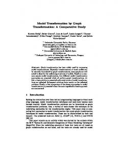
Figure 1: A Binary Asynchronous Control Structure and its State Transition Diagram We also denote the sets of input and output interconnections for a component v as: I H (v) = f(v0 ; v) 2 H g, and H O (v) = f(v; v0 ) 2 H g, respectively. The sets of input and output signals, or simply inputs and outputs, for a component are denoted: I Y (v) = fy : ?1 (y) 2 I H g, and OY (v) = fy : ?1 (y) 2 OH g, respectively.

A simple example of an ACS is described in Figure 1.(a). Here V = fa; b; cg, H = f(c; a); (a; c); (c; b); (b;c)g, Y = fRa ; Rb; Aa ; Abg, and (c; a) = Aa , (a; c) = Ra , (c; b) = Ab , (b; c) = Rb. Furthermore I H (c) = f(a; c); (b; c)g, I Y (c) = fRa ; Rbg, and so on. For every variable y 2 Y , S (y) = fy0 ; y1 ; :::; ykg is called the set of variable values, or states. An ACS hV; H; Y; i is called a Binary Asynchronous Control Structure (BACS) if 8y : S (y) = f0; 1g. Hence, for a BACS, the set of allowed changes can be denoted as Y  f+; ?g, where “+” stands for a signal change from 0 to 1, and

“-” for a signal change from 1 to 0. The behavior of a BACS is defined by a binary transition system, called state transition diagram, which is introduced in the following section.

2.2

Transition Systems and State Transition Diagrams

This section describes how the interconnected components of an ACS behave in time, that is how the variables associated with them change, using some key concepts from [9]. A Transition System (TS) is a pair hS; E i, where S is a set of states, and E; E  S  S , is a set of transitions. Note that we do not restrict S and E to be finite. The directed graph representation of a TS is as usual: states are vertices and transitions are arcs. For example, in Figure 1.(b) S = fs1 ; : : :; s13 g and E = f(s1 ; s2 ); (s1 ; s8 ) : : :g. We denote (s1 ; s2 ) 2 E by s1 Es2 . An Arc-Labelled Transition System (ALTS) is a quadruple hS; E; A;  i, where hS; E i is a TS, A is a finite alphabet of actions and  : E ! A is a (total) labelling function, which assigns each transition a single action name in A. Each action name represents a change of value of a variable in the associated ACS, and each (possibly infinite) path along the graph represents a valid sequence of such changes in time. Thus the ALTS describes the complete allowed behavior of the associated ? + ? + ? + ? + ACS. For example, in Figure 1 we have A = fR+ the change a ; Ra ; Aa ; Aa ; Rb ; Rb ; Ab ; Ab g, where we use Aa to denote + + of signal Aa from 0 to 1, and A? to denote the change from 1 to 0. Furthermore  ( s ; s ) = R ,  ( s ; s ) = R , 1 2 2 7 a a b and so on. For a BACS with a set of variables Y (jY j = n) we define a Binary (encoded) Transition System, or State Transition Diagram (STD), hS; E; i, where hS; E i is a TS and  : S ! f0; 1gn is a (total) labelling function such that each state is encoded with a binary vector consisting of the values of Boolean variables. The i-th component of the vector associated with each state s is denoted as (s)i , but for simplicity, unless it creates confusion, we generally use the simpler notation si . An STD is called contradictory if  is not injective. Hence for a non-contradictory STD we can identify the state with its binary label. For every STD arc, connecting a pair of states s and s0 , we allow s and s0 to differ in one and only one component, say the i-th. This component variable, yi , is called excited in state s and its value si is marked with a “*” in s. Since there can be several outgoing arcs from each state, a number of variables can be excited in it. The variables that are not excited in a state are called stable in it. We assume that transitions between the states can have arbitrary but finite delays, and that these delays are associated with the delays of the components in the modeled BACS (similar to the gate delay model in asynchronous circuits,

4

Section 3.2). We call an STD initialized if it has an explicit initial state. For example, in Figure 1.(b) Y = fRa; Aa ; Rb; Abg, and (s1 ) = 0000, (s5 ) = 1000 and so on. Furthermore, Ra and Rb are excited and Aa and Ab are stable in s1 . Note that every STD can be also interpreted as an Arc-Labelled Transition System, with the following labelling (consistent, since exactly one variable changes in every arc of an STD):

 + 8e = (s; s0 ) 2 E :  (e) = yyi? i

if si if si

0 and s0i = 1 and s0i =

= =

1 0

The following important property of any STD comes directly from its definition: Property 2.1 No state in an STD can have two outgoing transitions labelled with the same variable but with different signs. We can now examine more in detail the meaning of Figure 1. It represents the interconnection of an arbiter and two other components (the arbiter’s environment), that independently of each other may request access to a single resource, with signals, Ra and Rb. The arbiter grants access with Aa and Ab (which are mutually exclusive). Note that this BACS/STD pair specifies a fair behavior, because if the arbiter receives a request at one input, say Ra, while it is processing a previous request from Rb , then it must, after finishing the transaction for Rb, respond to Ra before it can react to a new request from Rb again. Our abstract arbiter is capable of distinguishing the order in which the two, possibly concurrent, requests arrive at its inputs, by going to two different states (s7 and s13 ), labelled with the same vector 1100 (hence the STD is contradictory). 2.2.1

Reachability and Unique Action Relations

Intuitively, a state s2 of a TS hS; E i is reachable from a state s1 if there exists a directed path from s1 to s2 . More formally, the direct reachability relation is simply given by the set E . For any pair of states s; s0 2 S , the state s0 is called reachable from s if there is a finite length (including zero length) sequence of transitions leading from s to s0 . Therefore reachability is given by reflexive and transitive closure of E , i.e. E  . In the example of Figure 1.(b) all states are mutually reachable. Similarly for any ALTS hS; E; A;  i we can define the reachability through a sequence of actions. Specifically, for direct reachability through action a; a 2 A, we have sE (a)s0 if sEs0 and  (s; s0 ) = a. For example in Figure 1.(b) we have s1 E (R+a )s2 . For general reachability through a sequence of actions, sE ()s0 would imply that there is a finite sequence of action names  2 A ;  = a1 ; a2 ; :::; am such that sE (a1 )s1 ; s1 E (a2 )s2 ; :::; sm?1E (am )s0 . We can sometimes use the + + notion of an allowed sequence from a state, i.e.  is allowed from s if 9s0 such that sE ()s0 . So R+ a ; Aa ; Rb is allowed in s1 , but it is not allowed in s2 in Figure 1.(b) Note also that among the various arcs labelled with the same action in Figure 1.(b), some of them actually represent exactly the same “event”. For example, arcs (s2 ; s3 ) and (s7 ; s6 ) both represent the same event, the arbiter acknowledging request R+ a from the environment. Now we make this intuitive idea more formal, because it will become important when we relate state-based models, such as the State Transition Diagram, with event-based models, such as the Signal Transition Graph, where the notion of unique occurrence of an event is explicit. For an ALTS hS; E; A;  i, we define a pairwise relation 1 on the set E of arcs as (s1 ; s01 ) 1 (s2 ; s02 ) if  (s1 ; s10 ) =  (s2 ; s02 ) and s10 6= s2 and s1 Es2 (i.e. there exists an arc (s1 ; s2 ) 2 E ). Let  be the equivalence relation formed by the reflexive, symmetric and transitive closure of 1 . We call  the unique action relation. We can easily see that Unique-Action Relation partitions the set E into a set of Unique-Action Relation-classes, [E ]A. Each such class, [e]a, is called an action. The set of actions with the same name, a, is called the action set of the name a and denoted as [E ]a. This notion will be useful later, when we shall associate the transitions of an STG with the transitions of the corresponding STD. For example, in Figure 1.(b) we have (s2; s7 ) 1 (s3 ; s6 ), and (s3 ; s6 ) 1 (s4 ; s5 ), hence, by transitivity, (s2 ; s7 )  (s4 ; s5 ). + Also (s1 ; s8 ) 1 (s2 ; s7 ). Then [e]Rb = f(s1 ; s8 ); (s2 ; s7 ); (s3 ; s6 ); (s4 ; s5 )g. In this very simple case, each action set has a + + single element, [E ]Rb = f[e]Rb g and so on. For an action [e]a , the set, always forming a connected subgraph, of states which are the sources for the transition arcs + in [e]a is called excitation region for action [e]a . So in Figure 1.(b) the excitation region of [e]Rb is fs1 ; s2 ; s3 ; s4 g, and they correspond to the states where the label bit for Rb has value 0 and is tagged with “*”. 2.2.2

Interleaving Semantics of Concurrent Actions

Throughout this paper we assume that the actions associated with a set of arcs outgoing from the same state can be performed + in the modeled system concurrently, i.e. independently of each other. See for example R+ a and Rb in s1 in Figure 1.(b), which are “produced” by different and independent components. Since our model is entirely asynchronous, we must assume that the changes of corresponding variables can occur in time in any order. 5

Our low-level behavioral model, on the other hand, requires that a single variable changes for every transition. We then choose to model such concurrency by interleaving, i.e. considering all possible alternative chain orderings compliant with the partial order between possibly concurrent actions (in Figure 1.(b) this corresponds to paths s1 ; s2 ; s7 and s1 ; s8 ; s13 ). Such a modeling is convenient yet sometimes problematic, because it hides the semantic distinction between true concurrency and “shuffled” alternative selections. This distinction can be made explicit only in models with explicit causality notions, and we postpone it until Section 4, where we will consider Signal Transition Graphs. 2.2.3

Properties of Transition Systems and State Transition Diagrams

In this section we analyze a set of behavioral properties of Transition Systems and State Transition Diagrams that we will show later been connected with corresponding, important properties of asynchronous systems. For example, the property of confluence below is closely connected to the requirement that the “long term behavior” of the system must not be influenced by the relative magnitude of the delay of two components. No matter who “wins the race”, we must still be able to reach the same state in the future. Similarly, local confluence will be shown to be related to the classical concept of static hazards in a circuit. Following [9], we call an ALTS hS; E; A;  i :

 

confluent, if 8s; s1; s2 2 S , if sE  s13 and sE  s2, then 9s3 2 S such that s1E  s3 and s2E  s3.

locally confluent, if 8s; s1; s2 2 S , if sEs14 and sEs2, where s1 6= s2, then 9s3 such s3 is unique, then the ALTS is called uniquely locally confluent.

2 S such that s1Es3 and s2Es3. If

So, Figure 1.(b) is confluent (all pairs of states can reach any state), but not locally confluent, due to s1 ; s2 and s8 (s1 Es2 ,

s1 Es8 , but there is no common immediate successor of s2 and s8 ).

Keller, in [9], gave three sufficient conditions for local confluence (and hence confluence) of an ALTS. An ALTS is:



deterministic, if 8s; s1; s2 2 S and 8a 2 A, if sE (a)s1 and sE (a)s2, then s1 only one outgoing transition from a state that is labeled with it).



commutative, if 8s 2 S and 8a; b 2 A, if ab and ba are allowed in s, then 9s0 such that sE (ab)s0 and sE (ba)s0 (i.e. if the effect of interleaving two transitions both allowed in a state and not mutually exclusive is the same).



persistent, if 8s 2 S and 8a; b 2 A; a 6= b, if a and b are allowed in s, then ab is allowed in s (i.e. if no transition can disable another one).

=

s2 (i.e.

for each action there can be

It was proven in [9] that if an ALTS satisfy all these conditions together, then it is both Locally Confluent and Confluent. The definition of STD implies that if an STD satisfies these conditions, then it is uniquely locally confluent. + The ALTS in Figure 1.(b) is deterministic and persistent, but not commutative (due to s1 ; R+ a and Rb again). So, being confluent, it shows that Keller’s conditions are only sufficient. Now, even though our state-based model has no “direct” idea of causality between actions, we can still locally verify if some action has “a unique set of predecessors”, that can somehow be identified with its causes. Hence we define the property of strict causality of an ALTS, which, as the Unique Action Relation, will become more clear when we introduce our event-based model, where such causality is explicit. Let S = hS; E; A;  i be an ALTS and let [E ]A be its set of actions. Let S ([e]a ) denote the excitation region for action a [e] 2 [E ]A . Let  (s1 ; s2 ) be a directed path of states between s1 and s2 . An ALTS is called strictly causal for action [e]a and state s 2 S if:

 8s1 ; s2 2 S ([e]a ); s1 6= s2 , such that 9(s; s1 ); (s; s2), with (s; s1 ) \ S ([e]a ) = ; and (s; s2 ) \ S ([e]a ) = ; (i.e. s1 is the first state in (s; s1 ) where [e]a is excited, and similarly for s2 ), –

9s3 2 S ([e]a ) (possibly coincident with s1 or s2 ) such that:  (s; s3 ) \ S ([e]a ) = ; and  9(s3; s1) such that (s3; s1)  S ([e]a ).

I.e. s1 and s2 have a common “ancestor”, through states where where [e]a is also excited for the first time. 3 I.e. s 1 4 I.e.

is reachable from s. there is an arc (s; s1 ) 2 E .

6

[ ]a

e

is also excited, which is a successor of s and

An ALTS is called strictly causal if it is strictly causal for all actions [E ]A in and all states in S . This definition means, informally, that each excitation region of each action has a single “top” state (or a “cycle” of such states, as in the example below), where it becomes excited for the first time, and all other states in the region (which is connected by definition) are successors of it through paths within the region. So actions leading into this “top” state (or cycle) can be informally identified with its causes. On the other hand, if the ALTS is not strictly causal, it means that some action has “many alternative ways” of becoming allowed. + The ALTS in Figure 1.(b) is strictly causal, because, for example, for action [e]Ra the states in its excitation region fs1; s2 ; s9; s10g form a cycle. So, for example, from state s4 we can reach both s1 and s8 (through s5 ), and in this case the third state in the definition coincides with s1 , whence s8 is reachable without leaving the excitation region. Similarly for all other triples of states and actions. Finally, when analyzing the behavior of an ALTS we are interested in checking if we have a point where future behaviors diverge completely. Such behavior is, in general, not desirable, and hence the liveness of an ALTS is important to check. We define it only for finite ALTS. For a finite ALTS, with the reachability relation E  between states, we define the mutual reachability relation between any two states, s; s0 2 S if both sE  s0 and s0 E  s hold for them. This is an equivalence relation, so it gives rise to a set of equivalence classes. Built for a given initial state, these classes form a partial order induced by the reachability relation. The maximal classes in this partial order are called final classes (i.e. once we enter one of these classes, we can never leave it). A finite ALTS is live if it forms a single equivalence class for any initial state. Such a TS is represented by a strongly connected graph. In a live ALTS, for every state s 2 S and every action name a 2 A, there exists a state s0 2 S , reachable from s, in which a is allowed. The ALTS in Figure 1.(b) is obviously live.

2.3

Trace Models

For an ACS defined by an ALTS we can define another representation, called Trace Structure, or Trace Model (see [22])5 , of its behavior. This representation will be needed in Section 5.3, because delay-insensitive circuits were defined in the literature using Trace Models, so in order to define delay-insensitivity within our framework we must relate Trace Models with Arc-Labelled Transition Systems. A Trace Model representation of the behavior (described by an Arc-Labeled Transition System) of a structure (described by a Binary Asynchronous Control Structure) is a pair hA;  i, where   A is a prefix-closed set of traces, or strings of actions. This model is defined with respect to a given initial state, and represents the execution history of the ALTS. Each trace then stands for a (possibly infinite) sequence of actions that can be performed on the variables of the ACS. The set of traces in  contains those traces that are allowed by the behavioral specification. For a BACS with an associated initialized STD and a set of variables Y , we can also think about a Binary Trace Model, which is a pair hY;  i, where   (Y  f+; ?g) is a prefix-closed set of traces, or strings of signal changes as allowed by the STD. ? + ? + ? + ? In the example in Figure 1, initialized in state s1 , we have A = fR+ a ; Ra ; Aa ; Aa ; Rb ; Rb ; Ab ; Ab g, and  = + + + + + + + + + + + + + f; Ra ; Rb ; Ra Rb ; Rb Ra ; Ra Aa ; Rb Ab ; Ra Aa Rb ; : : :g (here  stands for the empty trace). The following property of the Binary Trace Model generated from an STD is the result of Property 2.1 and of the definition of STD. Property 2.2 In a Binary Trace Model hY;  i, for every trace in  and any variable y 2 Y , all the occurrences of y have alternating signs, i.e. between any two consecutive changes of the same sign there is at least one opposite change.

2.4

Cumulative Diagrams

In order to characterize classes of behaviors of asynchronous systems, we need the concept of history of the execution of a state-based specification. The complete history of the system is represented by a set of traces, where each trace records exactly the order of occurrences of actions. The state of the Arc-Labeled Transition System, on the other hand, describes only the final result of such execution. In this section, following [16], we will describe a model to describe this history, where only the number of occurrences of each action is recorded, called a Cumulative Diagram (CD). Hence this representation will be of intermediate “precision” between a Trace Model and an ALTS. The Trace Model description of the operation of an initialized ALTS contains all the traces of the ALTS starting from its initial state. The mechanism of trace generation induces a natural mapping between traces and sets of states, where each trace 5 We are forced to introduce this term here, as a synonym of the more common “Trace Structure”, only to avoid confusion with the abbreviation of the term “Transition System” (TS).

7

Ra+ Aa+ RaAaRa+ Aa+

2020

3020

2120

3130

3120 Ab+ 3121

Ra- 3030

Rb+

1100

0100 Ab+ 0101

Rb-

1101

0201 Ab-

1000

1010

2010

0000

1110 2110

1201

2121

1212 2212

2221

Rb- 3221 Ab- 3222

2222

2312 Aa2322

0202 Rb+ 0302 Ab+ 1202 1302 0303 1312 Aa+ 1303 Ra-

Rb-

Figure 2: The Cumulative Diagram of Figure 1 maps to the set of states where the ALTS may be at the end of its generation. Note this mapping is functional if the ALTS is deterministic. In this case, the state in which the ALTS arrives for a given trace with respect to an initial state is uniquely determined through the reachability relation. On the other hand, for any ALTS (not just deterministic ones) we can think about another mapping from the set of traces. This mapping defines, for every trace  2  , a multiset of action names , with the multiplicity of each name a 2 A, (a), equal to the number of occurrences of a in . A multiset obtained in this way is called a cumulative state. It is convenient to represent a cumulative state by a vector of natural numbers with dimension jAj. We can easily see from the above definition that a cumulative state defines a class of equivalence between traces of the ALTS which are simple permutations of each other (note that not every permutation may be a valid trace). Let [] be such equivalence class for trace . Every trace 2 [] brings the ALTS to the same cumulative state . Therefore we can identify this  with []. Now it should be clear that for every deterministic, commutative and persistent ALTS, where all the traces in [] bring the ALTS in the same state, there exists a functional mapping between cumulative states and ALTS states. The set of cumulative states generated by an ALTS through its Trace Model model (denoted by [ ]) is a partial order. This order is a subset of the natural integer vector ordering and is built upon the prefix order between traces up to permutations. Formally, [] v [ ] if there exist  2 [] and 2 [ ] such that  is a prefix of . The partial order of cumulative states, built as above, is called the Cumulative Diagram (CD) (more precisely, we will use its Hasse diagram, where the reflexive and transitive edges have been removed). For example, Figure 2 contains an initial fragment of the CD for the ALTS described in Figure 1. Note that the CD model cannot describe the local divergence after traces Ra + Rb+ and Rb + Ra+. In fact both traces lead to the same cumulative state 1100, that corresponds to states s7 and s13 in Figure 1.(b). This also illustrates that the mapping between CD states and STD states in general is a relation, not a function. The above definitions are easily adapted to the case of a BACS and its STD. By Property 2.1, we can change the notion of cumulative state and build the CD for a set of variable names Y rather than their changes Y  f+; ?g. This modified version of CD is isomorphic to the original version because all the changes of the same variable are linearly ordered (see also Property 2.2). Now we have all the necessary information to define the notion of speed-independent and semi-modular behavior, which are crucial (as we will see in Section 3.6) for more practical purposes, such as the analysis and synthesis of asynchronous control circuits.

2.5

Speed-independence and Semi-modularity

The intuitive notion of speed-independent behavior can be more formally described using confluence, that ensures that the “long term” behavior of the modeled asynchronous system does not depend on the winner of a race between concurrent transitions. In this section we give a set of alternative definitions of a set of ALTS properties. These properties will be shown to correspond to:

 

interesting circuit properties, such as the absence of hazards in Section 3, and high-level specification properties in Section 5.

8

So this section provides the desired bridge between the two domains. Let us first recall some definitions from lattice theory. Let C be a partial order. An element z 2 C is a zero element if for all c 2 C we have z v c. An element c 2 C is a greatest lower bound (g.l.b.) of two elements c1 ; c2 2 C , denoted c = c1 u c2 , if c  c1 , c  c2 and c0  c1 ^ c0  c2 ) c0  c. Similarly we can define the least upper bound (l.u.b.) of a pair of elements, denoted c = c1 t c2 by replacing  with . A lattice is a partial order where every pair of elements has a g.l.b. and a l.u.b.. A lattice is distributive if the g.l.b. and l.u.b. operations are mutually distributive. An element c1 of a partial order C covers another element c2 of C if c2  c1 and there is no c3 such that c2  c3  c1 . A lattice is semi-modular if for every pair of elements c1 and c2 that cover a third element c3 (then obviously c3 = c1 u c2 ), they are both covered by c1 t c2 .

  

An ALTS (STD) is called Speed-independent-1 if it is confluent. A finite ALTS (STD) is called Speed-independent-2 with respect to a state if the CD generated for this state is a lattice with a zero element, according to the partial order defined in Section 2.4. The ALTS (STD) is called Speed-independent-2 if it is Speed-independent-2 with respect to every state in S . A finite ALTS (STD) is called Speed-independent-3 ([18]) with respect to a state s if it has a single final equivalence class when initialized in s (Section 2.2.3). The ALTS (STD) is called Speed-independent-3 if it is Speed-independent with respect to every state in S .

For example, the ALTS in Figure 1.(b) satisfies Speed-independent-3, because it is finite and it has a single final equivalence class for every initial state. We can easily see that the TS is confluent, and hence Speed-independent-1. Furthermore its CD, represented in Figure 2, is a lattice (zero is cumulative state 0000), so the STD is Speed-independent-2. It can be shown that, despite our intuition, the definitions above are not strictly equivalent for a given finite ALTS (STD). Speed-independent-1 is equivalent to Speed-independent-3 in the finite case, while Speed-independent-1 and Speedindependent-2 are equivalent if (but not only if) the given finite ALTS (STD) is deterministic, commutative and persistent: Proposition 2.1

 

A finite ALTS (STD) is Speed-independent-2 if it is Speed-independent-1 and persistent. An ALTS (STD) is Speed-independent-1 if it is Speed-independent-2, deterministic and commutative.

The example in Figures 1 and 2 shows that our conditions for the equivalence between Speed-independent-1 and Speedindependent-2 are only sufficient and not necessary, because this ALTS is both Speed-independent-1 and Speed-independent-2 but not commutative. Semi-modularity, that we will relate to hazard-freeness, is a stronger property than speed-independence. Again, two alternative definitions can be formulated.

 

An ALTS (STD) is called Semi-modular-1 if it is locally confluent. A finite ALTS (STD) is called Semi-modular-2 with respect to a given state if the CD generated for this state is a semi-modular lattice with a zero element, according to the partial order defined in Section 2.4. The ALTS (STD) is Semi-modular-2 if it is Semi-modular-2 for every state in S .

A Proposition analogous to Proposition 2.1 can also be shown to hold about Semi-modular-1 and Semi-modular-2. The ALTS in Figure 1.(b) is not locally confluent, hence not Semi-modular-1. It is not Semi-modular-2 either, because the corresponding CD in Figure 2 is not semi-modular, due for example to cumulative states 1110 and 1101, that both cover 1100, but are not covered by their least upper bound 2222 (recall that covering means being immediately above in the partial order). A last class of ALTSs, significant because of some interesting results on sufficient conditions for its synthesis with realistic logic gates ([25]), is connected with the definition of strict causality (or, informally, of a “unique set of actions causing an action”) described in Section 2.2.3.

 

An ALTS (STD) is called Distributive-1 if it is strictly causal and locally confluent. A finite ALTS (STD) is called Distributive-2 with respect to a given state if the CD generated for this state is a distributive lattice with a zero element, according to the partial order defined in Section 2.4. The ALTS (STD) is Distributive-2 if it is Distributive-2 for every state in S .

A Proposition analogous to Proposition 2.1 can also be shown to hold about Distributive-1 and Distributive-2. It should be obvious that the following inclusion holds for the classes of ALTSs (STDs): Distributive  Semi-modular  Speed-independent. 9

#(z1,z2,z3)

z1 z3

z1 z2 z3

000

z2

+z1

0*0*0

1 0*0* +z2 +z3 -z2

100

+z2

0*1 0*

+z1 1 1 0* +z3

(a) -z3 302

-z2

303

211 212

312 213

0 0 1* ...

...

(b)

011

111

202

0 1* 1 -z1

110

201

+z3

1*1*1 -z1

1*0 1

101

010

223 ...

021 121

221 222

022 122

032

123 132

... ...

...

033 ...

(c)

Figure 3: A circuit, its State Transition Diagram and its Cumulative Diagram with Inertial Delays

3

Modeling Asynchronous Logic Circuits

In this section we will show how “real” asynchronous circuits, built out of gates and wires, fit as a special case of our Binary Asynchronous Control Structures and State Transition Diagrams. We will use two different delay models, pure and inertial, to describe the behavior of the circuit, and characterize circuit properties such as hazards in terms of ALTS properties such as local confluence.

3.1

A Low-level Model for Asynchronous Logic Circuits

Here, as in Section 2.1, we describe a circuit as the conjunction of a structure (a graph) and a behavior (a set of Boolean functions and delays). An Asynchronous Logic Circuit (ALC, [18], [16]) is a triple hX; Z; F i, where X is a set of input signals (jX j = m), Z is a set of output signals (jZ j = n), F = ff1 ; f2 ; :::; fng is a set of Boolean functions, the circuit element functions, such that for each i 2 f1 : : :ng; fi : f0; 1gdi ! f0; 1g, where di is the number of inputs of element zi . We denote by Y = X [ Z , the set of signals of the ALC. The structure of an ALC can be represented by a directed graph with one node for each variable, and an arc connecting the node corresponding to each input of fi with the node corresponding to yi 6 . Structurally, an ALC is a special case of a BACS. The difference is that every structural component of the ALC is uniquely associated with a single variable, thus implying that each component, vi , has only one output, fyi g = OY (vi ). The value of this output can be characterized either by the value of the corresponding Boolean function fi (if yi is an output signal) or by the value of the signal itself (if yi is an input signal). An ALC is initialized if its initial state is defined, as a binary vector s0 2 f0; 1gn+m. An ALC is autonomous if X = ;. Figure 3.(a) describes a very simple autonomous ALC, where Z = fz1 ; z2 ; z3 g and f1 = z3 ; f2 = z3 ; f3 = z1 + z2 .

3.2

Taxonomy of Models for Asynchronous Logic Circuits

An initialized ALC produces a dynamic behavior, resulting from the transitions of both input and output signals. The input signals are changed by the environment and the output signals are changed by the ALC. The output values are determined by two factors. The first factor is the evaluation of the Boolean function associated with the element. The second factor is the inherent switching delay of the physical logic gate, which must be taken into account by the model. Therefore the dynamic behavior of the ALC is modeled through a number of abstractions, which can be classified as follows: 1. Delay model of an element (delay model “in small”, see Section 3.3):



pure delay model,

6 We associate a node with each input of an ALC to provide the way of modeling the input wires of the circuit as components with potential delay properties.

10



inertial delay model.

2. Delay model of the circuit (delay model “in large”):

  

feedback delay model ([8]), assuming that there are delays only in the feedback wires. gate delay model, ([18]), assuming that only the logic elements have finite delays. gate and wire delay model, ([3] and [4]) assuming that both gates and wires have finite delays.

3. Environment behavior model (input change constraints):

 

fundamental mode, assuming that inputs can change their values only after the circuit has reached a stable state, where none of its variables is excited. input-output mode, allowing the environment to change the input values in some states, not necessarily stable, in accordance with some protocol of interaction between the ALC and the environment. The fact that input values may change in some states, autonomously or in consequence of some output change, is explicitly indicated in the model (reactive behavior).

4. Circuit switching semantics (“race” model):

 

general multiple winner, assuming that any subset of the set of unstable signals may win the race due to a concurrent switching process. extended multiple winner, where all concurrently changing signals go through a third, undefined, state before reaching their final value.

Brzozowski and Seger ([3]) showed that General Multiple Winner and Extended Multiple Winner yield equivalent results, but the latter allows more efficient analysis of the circuit hazards than the latter. Ternary simulation, can be used to analyze a circuit with the Extended Multiple Winner model, but only in a rather limited case, the Fundamental Mode operation. The ternary simulation of the dynamic behavior of an ALC in I/O mode (or of an autonomous ALC) cannot give meaningful results for such effects like hazards or speed-independence7 . Due to these reasons our analysis assumes the General Multiple Winner race model and I/O mode.

3.3

Delay Models of an Asynchronous Logic Circuit element

Let an ALC hX; Z; F i be initialized in some state s. Every element zi of the circuit is modeled as a sequential composition of a delay-free logic function evaluator and a delay block. For every element zi we call it (and the corresponding output variable) stable in s if its current value si is equal to the value of its function fi . Otherwise we call it excited. We assume that if a variable is excited, then this variable may change its state after some finite time interval, which we call the element delay. For example, in the circuit in Figure 3.(a), initialized in state 000, z3 is stable while z1 and z2 are excited. What happens next, whenever z1 or z2 changes value, depends on whether we use the pure or inertial delay model. 3.3.1 Inertial Delay Model In the Inertial Delay model (ID), an excited variable may change its state after a finite delay. This means that for any excited variable zi there are two possibilities. One is that its value, 0 or 1, changes to the opposite, i.e. to 1 or 0, after a finite but unbounded amount of time. The other possibility is that the value of its function fi is changed before zi manages to change, so that the previous value appears at the input of the delay block. In this case the output zi of the element ceases to be excited and retains its previous value, which becomes stable (hence the term “inertial”). Speaking in more quantitative terms, the ID model means that if an element has a switching delay of d time units, pulses generated by the logic evaluator with duration less than d are filtered out, while pulses longer than d units appear at the output zi shifted in time by d units. Since we are dealing with completely asynchronous circuits, we cannot precisely say whether in the second situation above the element has or has not produced a short pulse at its output. We shall therefore regard this behavior (when fi changes before zi ) as anomalous or hazardous. 7 Although some results on speed-independence can be obtained through such technique [3], they are meaningful only for a very restrictive modeling conditions. Namely, the circuit must operate in Fundamental Mode, and it is regarded as Speed-independent if its final equivalence class consists of a unique stable state. The existence of cyclic final equivalence classes cannot be detected by such ternary simulation, because each cyclically changing variable would have an undefined value.

11

3.3.2 Pure Delay Model We can alternatively assume that the delay block of each element is not inertial when it becomes excited, i.e. it cannot filter out the pulses whose duration is less than a given value d (this behavior is close to reality for long wire delays). Therefore, even though the function value changes before the output zi has changed, the element remains excited, and just shifts in time the complete sequence of its “expected” output transitions. With this Pure Delay model (PD), the value of the element in state s of the ALC, must be modeled by a pair, (ris ; is), where the first component is the current binary value of zi , i.e. ris 2 f0; 1g, while the second component is the excitation number (recording how many excitations have been registered by the functional evaluator since the element was last stable), is 2 f0; 1; 2; :::g. In this model, the state of the ALC is a vector of length jY j, with each component being of the above form. We can now define an element zi to be stable, according to the PD model, in state s if is = 0. Otherwise it is excited. The normal operation of the element is described by the following sequence of transitions: (ris ; 0) ! (ris ; 1) ! (ris ; 0). The hazardous operation, on the other hand, is described by the following sequences of transitions: either (ris ; is) ! (ris ; is + 1) ! (ris ; is ) (if is > 0) or (ris ; is ) ! (ris ; is + 1) ! (ris ; is + 2). Now, with this definition of the behavior of each gate, we can describe the operation of the entire circuit for both the ID and the PD models.

3.4

Circuit Behavior Description with Inertial Delays

Let us consider, as an example, the circuit shown in Figure 3.(a). If we assign the all zero vector as the initial state of this ALC, variables z1 and z2 are excited in this state. As usual, we designate this fact by labelling the value of an excited variable with an asterisk (*). Therefore the initial state is marked as 0 0 0. Using the ID model of an element we can think about two possible states directly reachable from this state through the element normal switching behavior, 100 and 0 10 . Although variables z1 and z2 are excited concurrently and can switch independently, our interleaving semantics of concurrent actions requires that the first of the above two states is reached if variable z1 changes before z2 (and vice-versa). In both cases variable z3 now becomes excited. We can thus use a depth-first search procedure to generate the set of states reachable from the initial state. This set, together with the relation of direct reachability between states, can be represented by a graph, which satisfies our definition of an STD. Note that the transitions in this graph are labelled by the changes of variable values. Since the number of signals in the ALC is fixed (jY j = n + m), it is obvious that the size of the STD, in terms of the number of its state labels, is bounded by 2n+m . Proposition 3.1 The STD for any ALC, under the ID element model, is deterministic, commutative and non-contradictory8. This Proposition follows directly from the ID model of an element and the uniqueness of the result of Boolean function evaluation for any given binary encoded state. Therefore determinacy and commutativity are the intrinsic properties of the STD description for any ALC obtained using the ID model. This implies that confluence and local confluence are determined (up to sufficiency) by how the circuit satisfies the persistency condition. We can now define speed-independence, semi-modularity, and so on for an ALC modeled with Inertial Delays. Let C = hX; Z; F i be an ALC modeled with inertial delay and let S = hS; E; i be its associated STD. According to the classification of Section 2.5 and Proposition 3.1: 1. 2. 3. 4.

C is Speed-independent if the STD S is confluent. C is Output-persistent if it is Speed-independent and for each pair of edges s1 E (y1 )s2 and s1 E (y2 )s3 , if y1 2 Z , then y1 is enabled in s3 (i.e. no output signal can ever be disabled).

C is Semi-modular if the STD of S is locally confluent. C is Distributive if the STD of S is strictly causal and locally confluent.

Analogous definitions exist for a BACS (except for Output-persistent). Output-persistency guarantees that no transition of an output signal will ever be disabled, thus guaranteeing a correct behavior for them (recall that disabling a transition means possibly causing a spurious pulse on the signal). Obviously ID-DistributiveID-Semi-modularID-Output-persistentID-Speed-independent. 8 Being

non-contradictory, we can identify each state of the STD with its unique binary vector code.

12

Note that Semi-modular as defined above is equivalent to the “operational” definition due to Muller ([18]). An ALC is called Semi-modular with respect to a given state if the STD built from this this state has no transition from a state where some zi is excited to another state where zi is stable but has the same value. So an ALC is Semi-modular if its STD is persistent. Also, note that Proposition 2.1 and 3.1 immediately imply that for an ALC with the ID model Speed-independent1 (confluence) is implied by Speed-independent-2 (lattice), and similarly for Semi-modular-1 and Semi-modular-2 and Distributive-1 and Distributive-2. The STD and an initial fragment of the CD for the ALC example in Figure 3.(a) is shown in Figure 3.(b) and (c). The STD is live, Speed-independent but not Semi-modular (persistency is violated in states 1 01 and 011, where z2 and z1 are disabled after the transition z3+ from states 10 0 and 0 10, respectively). It is confluent but not locally confluent. Furthermore it is strongly connected, thus having single final equivalence class, and it contains only non-transient cycles of states. The CD is a lattice (one can easily prove that every pair of cumulative states has its least upper bound in the CD), but not semi-modular. It has a zero element, the empty multiset (or all zero vector).

3.5

Circuit Behavior Description with Pure Delays

Throughout this section we will refer to properties of the ALC under consideration when analyzed with the Inertial Delay modes by prefixing them with ID. Properties without the prefix, on the other hand, refer to the ALC analyzed with the Pure Delay model. An Asynchronous Logic Circuit can be analyzed with the Pure Delay model in a similar way as in the Inertial Delay case, by building its CD with a depth-first search procedure, from the initial state. According to the notation introduced earlier, each state, s, is labelled by a vector of jY j = n + m pairs (ris ; is), where the first component is the binary value on the output of the delay block, zi , and the second component is the number of potential changes that the element will generate on its own before it will become stable. Let us call such a vector the PD-vector. This graph does not satisfy the definition of an STD, given in Section2.2, because the label is not binary. Nevertheless, it satisfies the definition of an ALTS, and again, due to the unique evaluation of the Boolean functions describing the ALC, we can make use of the fact that every state in set S is uniquely labelled by the PD-vector, and show that the following Proposition holds. Proposition 3.2 The ALTS for any ALC, under the PD element model, is deterministic, persistent and non-contradictory. Equality between PD-vectors requires also equality of the second component, so commutativity does not hold in this case. However, due to non-inertiality of elements behavior, we can claim persistency, because every element records its excitation, and cannot be disabled by changing the value at the output of its Boolean evaluator. The latter detail drastically changes the role of the CD that can be built from the ALTS associated with the ALC. Such a CD is no longer a description that can be meaningfully used for characterizing the confluence properties of the ALC behavior. The definition of a bounded circuit becomes crucial in such characterization. The PD model of an ALC (PD-ALC) is called k-bounded (or simply “bounded”) if for every reachable state s in the associated ALTS, 8zi : is  k. An immediate consequence of boundedness is the finiteness of the ALTS of a PD-ALC. The following Proposition is the implication of the fact that a PD-modeled ALC can accumulate unbounded “switching events” in its elements if its operation is cyclic. Proposition 3.3 The PD model of an ALC, which is ID-live9 and non-ID-persistent, is unbounded. This is true because in a live, non-persistent ID model of a circuit there is no bound to the number of times the circuit can reach a state s where a variable yi becomes disabled before it has a chance to fire. So every new arrival in this state will increment the corresponding is.

  

The PD model of an ALC is called Speed-independent if the associated ALTS is finite and confluent. The PD model of an ALC is called Semi-modular if the associated ALTS is finite and locally confluent. The PD model of an ALC is called Distributive if the associated ALTS is finite, strictly causal and locally confluent.

Analogous definitions exist for a BACS. This definition and Proposition 3.3 imply the following important result. Theorem 3.4 The PD-model of an ALC, which is ID-live, is PD-Speed-independent iff it is ID-Semi-modular10. 9 I.e. 10 I.e.

the STD of the same circuit, modeled with Inertial Delays, is live. That is, it forms a single equivalence class for any initial state (Section 2.2.3). the same circuit modeled with Inertial Delays is Semi-modular.

13

z1 z2 z3 (0,1)(0,1)(0,0) +z1 +z2 (1,0)(0,1)(0,1)

(0,1)(1,0)(0,1) +z1

+z3

+z3 +z2 (1,1)(0,2)(1,0) (1,0)(1,0)(1,1) +z2 +z3 -z1 (0,0)(0,2)(1,1) -z3

(0,2)(1,1)(1,1)

(1,1)(1,1)(1,0) +z2

-z2

+z1 -z2

-z1

... ((1,1)(0,0)(1,0)

(0,0)(1,1)(1,2) (0,1)(0,3)(0,0) +z2 +z1 -z3 -z2 (1,0)(0,3)(0,1) +z3

+z2

(1,1)(0,4)(1,0) ...

...

(0,1)(1,2)(0,1)

(0,0)(1,1)(1,0) -z1 -z2 (0,0)(0,0)(1,3) (0,0)(0,0)(1,1)

+z3 -z2 +z1 (1,0)(1,2)(0,1) (0,2)(1,3)(1,0) ...

...

...

...

-z3

-z3 (0,1)(0,1)(0,2) ...

...

...

Figure 4: Cumulative Diagram for Pure Delay Model This theorem in practice claims that for the PD model of an asynchronous circuit, speed-independence amounts to semimodularity, if one considers a cyclically operating circuit. This result provides a crucial justification for the restriction to semi-modularity, when we look for necessary and sufficient conditions for the hazard-free, speed-independent implementation of an ALC. Note also that this equivalence result strongly favors the use of semi-modularity rather than speed-independence as the characterization of a “correct” circuit in the ID case. The ID model can be too optimistic in many practical cases, so a design made for semi-modularity (or output-persistency) will be more “robust” with respect to technology changes, different implementations of other components of the system, and so on. Obviously PD-DistributivePD-Semi-modular. Our ALC example in Figure 3.(a) generates the ALTS whose initial fragment is shown in Figure 4. This ALTS is persistent but non-commutative. It is infinite and not locally confluent. The PD-ALC is unbounded, therefore it is not Speed-independent. Our analysis of ID and PD models of ALCs has an important by-product. It gives concise and general characterization of hazards in the ALCs behavior.

3.6

On Static and Dynamic Hazards of Asynchronous Logic Circuits

The traditional definition of hazards ([21]) assumes two types of hazards, static and dynamic. Static hazards are again of two types, 0-1-0 and 1-0-1, and they model the behavior of an element which generates spurious pulse at its output. The dynamic hazards, 0-1-0-1 and 1-0-1-0, model the erroneous behavior of an element that should switch from 0 to 1 or 1 to 0, respectively, but during this process returns back to its previous state. Leaving aside the question of how dangerous such hazards are in an asynchronous context, we can identify how this behavior can be analyzed at our ID and PD modeling level. For a given ALC, the ID model, represented by the STD, can only depict static hazards. They are present if the ID-ALC is non-persistent. An element whose excitation is disabled, without switching, in state 0(1) is defined to have an 0-1-0 (1-0-1) static hazard11 . Hence, if the ALC is ID-Semi-modular (or ID-Output-persistent), then it is free from hazards. For a given ALC, the PD model, represented by its ALTS, can describe all hazards, characterized as follows. An element whose excitation number is is greater than 1 has a hazard. The rank, k, of this hazard is equal to is . This characterization allows us to define not only “standard” static or dynamic hazards, but any dynamic hazardous behavior that can be generated by the circuit element. In fact, the “standard” static hazard corresponds to is = 2, while the “standard” dynamic hazard to is = 3. 11 Strictly speaking, this is not a hazard in the “ideal” model, because the output of the delay block does not change. Due to the physical considerations above, though, this kind of situation can actually generate a spurious pulse on the output.

14

4

A High-level Behavioral Model for Asynchronous Systems

The previous Sections discussed various inter-related models of Asynchronous Control Structures and Logic Circuits, and the relationship between model properties, such as confluence, and circuit properties, such as hazards. In this section we develop a very general, event-based, model of BACS and ALC that, unlike STDs and Trace Models, has an explicit notion of causality and concurrency. So for example we will be able to distinguish the cases where events a and b are truly concurrent, independent of each other, and the case where either a can happen, and then cause b, or b can happen, and then cause a (an example of this distinction will be given in Figure 6). The model, called Signal Transition Graph (STG), is based on interpreted Petri nets, and is a development of similar, but less general, models presented by [19] and [5]. We first recall some basic definitions from the theory of Petri nets then establish relationships between STGs and the models described in the previous Sections.

4.1

Petri Nets

Petri nets are a widely used model for concurrent systems, because they have a very simple and intuitive semantics, that directly captures concepts like causality, concurrency and conflict between events. A Petri net (PN) is a triple P = hT; P; F i. T is a non-empty finite set of transitions. P is a non-empty finite set of places F  (T  P ) [ (P  T ) is the flow relation between transitions and places12. A PN marking is a function m : P ! f0; 1; 2; : ::g, where m(p) is called the number of tokens in p under marking m. A marked PN is a quadruple P = hT; P; F; m0 i, where m0 denotes its initial marking. A transition t 2 T is enabled at a marking m if all its predecessor places are marked. An enabled transition t may fire, producing a new marking m0 with one less token in each predecessor place and one more in each successor place (denoted by m[t > m0 ). A sequence of transitions and intermediate markings m[t1 > m1 [t2 > : : :m0 is called a firing sequence from m. The set of markings m0 reachable from a marking m through a firing sequence is denoted by [m >. The set [m0 > is called the reachability set of a marked PN with initial marking m0 , and a marking m 2 [m0 > is called a reachable marking. A PN marking m is live if for each m0 2 [m > for each transition t there exists a marking m00 2 [m0 > that enables t. A marked PN is live if its initial marking is live. A marked PN is k-bounded (or simply “bounded”) if there exists an integer k such that for each place p, for each reachable marking m we have m(p)  k. A marked PN is safe if it is 1-bounded. A transition t1 disables another transition t2 at a marking m if both t1 and t2 are enabled at m and t2 is not enabled at m0 where m[t1 > m0 . A marked PN is persistent if no transition can ever be disabled at any reachable marking. A PN is a Marked Graph if every place has exactly one predecessor and one successor. A Marked Graph is persistent for every initial marking m0 , furthermore every strongly connected marked graph has at least one live and safe initial marking. A PN is free-choice if any two transition with a common predecessor place have only one predecessor. A marked Petri net P = hT; P; F; m0 i generates an Arc-Labeled Transition System (ALTS) ([m0 >; E; T;  ) (Section 2.2) as follows. For each edge (m1 ; m2 ) 2 E , where m1 [t > m2 , we have  (m1 ; m2 ) = t. Under this mapping, each UniqueAction Relation-class [e]t, with e = sE (t)s0 corresponds to a particular firing of a transition t. The following Proposition is an obvious consequence of the PN firing rule and of the results in [9]: Proposition 4.1 1. The ALTS corresponding to a marked PN is finite if and only if the PN is bounded. 2. The ALTS corresponding to a marked bounded live PN is live. 3. The ALTS corresponding to a marked PN is deterministic and commutative. 4. The ALTS corresponding to a marked persistent PN is persistent, locally confluent and confluent. 4.1.1

Cumulative Diagram of a Petri Net

As in Section 2.4, we can define the Cumulative Diagram (CD) of a Petri net, and analyze its properties as a lattice. This will be useful in order to establish the desired correspondence between PN properties and circuit properties. According to [26], we define the Cumulative Diagram of a marked PN as follows. Given a firing sequence m0 [t1 > m1 [t2 > : : :m of a marked PN P = hT; P; F; m0i, the corresponding firing vector is a mapping V : T ! f0; 1; 2; :: :g such that for each transition t, V (t) is the number of occurrences of t in the sequence. 12 A

PN can be represented as a directed bipartite graph, where the arcs represent elements of the flow relation.

15

Let V be the set of all firing vectors of P . We define a mapping  : V ! [m0 > that associates each firing vector with the final marking of the corresponding firing sequence. Note that the mapping is well defined, since in any marked PN the marking reached after a sequence of transition firings from m0 depends only on the number of occurrences of each transition in the sequence, not on the order of occurrence. The set V , called the Cumulative Diagram of P , was shown in [26] to be a partial order when we define V1 v V2 if:

 V1 (t)  V2 (t) for all t and  marking (V2 ) is reachable from marking (V1 ). The following Theorem was proved in [2]:

Theorem 4.2 The ALTS of a PN is confluent if the net is free-choice, bounded and live. The following Theorems were proved in [26]: Theorem 4.3 The CD of a marked PN is a semi-modular lattice with a zero element if the net is persistent. Theorem 4.4 1. The CD of a marked PN is a distributive lattice with a zero element if the net is safe and persistent. 2. The CD of a Marked Graph is a distributive lattice with a zero element. 3. Let P be a PN whose CD V is distributive. There exists a safe and persistent PN with the transitions of P and whose CD is isomorphic to V .

P 0 whose transitions are labelled

4. Let P 0 be a safe persistent PN, let V be its CD. There exists a safe Marked Graph P 00 whose transitions are labelled with the transitions of P 0 and whose CD is isomorphic to V .

5. Let S be a finite distributive ALTS with a set of labels T . There exists a safe persistent PN P and a safe Marked Graph P 00 whose transitions are labelled with those in T and whose CDs are isomorphic to the CD generated by S .

4.2

Signal Transition Graphs

Interpreted Petri nets, where transitions represent changes of values of circuit signals, were proposed independently as specification models for Asynchronous Logic Circuits by [19] (where they were called Signal Graphs) and [5] (where they were called Signal Transition Graphs, STGs). Both papers proposed to interpret a PN as the specification of an ALC C = hX; Z; F i (where Y denotes, as usual, (X [ Z ),?by labelling each transition with an element of Y  f+; ?g. A+label ?yi+ means that signal yi 2 Y changes from 0 to 1, and yi means that yi changes from 1 to 0, while yi denotes either yi or yi . An STG is a quadruple G = hP ; X; Z;
i where P is a marked PN, X and Z are (disjoint) sets of input and output signals respectively and
: T ! (X [ Z )  f+; ?g labels each transition of P with a signal transition. An STG is autonomous if it has no input signals (i.e. X = ;). Both [19] and [5] gave also synthesis methods to translate the PN into an STD (called Transition Diagram in [19] and State Graph in [5]) and hence into an ALC implementation of the specified behavior. Given an STG G = hP ; X; Z;
i and the ALTS ([m0 >; E; T;  ) corresponding to its PN P , we define the associated STD S = h[m0 >; E; i as follows. For each m 2 [m0 >, we have (m) = sm , where sm is a vector of signal values. Let smi denote the value of signal yi in marking m. Obviously the STD labelling must be consistent with the interpretation of the PN transitions, so we must have for all arcs e = (m; m0 ) in the STD:

 if
( (e)) = yi+ , then smi = 0 and smi  if
( (e)) = yi? , then smi = 1 and smi  otherwise smi = smi .

0

0

=

1.

=

0.

0

Figure 5 shows an example of an STG and the corresponding STD. Note that for historical reasons PN transitions are denoted by the corresponding labels and PN places are denoted by circles PN places with only one predecessor and one successor are generally omitted. So in Figure 5.(a) the initial marking of the PN (corresponding to the leftmost state in Figure 5.(b)) appears on the edge between y? and x+ . An STG is defined as valid if its STD is finite (i.e. the PN is bounded) and has a consistent labeling. In this paper we will only consider valid STGs (otherwise their interpretation as control circuit specifications would lose its meaning). One consequence of this requirement is similar to Property 2.1: 16

z+

xz-

x+

0*00

y+

y+

y+ z+

110*

y-

y-

xx+ z+ 10*0* 1*0*1 00*1 y+ x011*

1*11

(a)

z-

01*0

(b)

Figure 5: A Signal Transition Graph and its State Transition Diagram

xz+

y+

y+

z+

z-

x+ yFigure 6: A Persistent Signal Transition Graph with non-persistent underlying Petri net Property 4.1 In a valid STG, for all firing sequences of its PN, the signs of the transitions of each signal alternate. Two STG markings m1 and m10 are equivalent if for each finite firing sequence m1 [t1 > m2 [t2 > : : : there exists a firing sequence m10 [t10 > m02 [t20 > : : : such that
(ti) =
(t0i) for all i. This relation partitions the set of reachable markings into equivalence classes. The equality between STG markings (and hence STD states) in the following will always be modulo this equivalence13 . An STG is persistent if for each reachable marking m1 , if t1 is enabled in m1 and m1 [t2 > m2 , with
(t1 ) 6=
(t2 ), then there exists a transition t3 enabled in m2 such that
(t1 ) =
(t3 ). An STG is output persistent if the above definition holds for all t1 such that
(t1 ) 2 Z . Note that this definition of STG persistence allows a case like that in Figure 6 to be treated as persistent, even though the underlying PN is not persistent. So PN persistency is a stronger condition than STG persistency. Only the transition labeling
that maps two different PN transitions into y+ (and similarly for z + ) “erases” the distinction that was present between the PNs underlying Figures 6 and 5.(a), so that the two STGs generate isomorphic STDs. This Figure illustrates clearly the “semantic gap” arising from using a purely interleaving semantics (as in the STD) versus using a true concurrent semantics (as in the STG). The following Theorem is a direct consequence of the results in [26]: Theorem 4.5 1. For every deterministic, commutative and persistent STD S there exists an STG whose PN is persistent, bounded and generates S .

2. For every distributive STD S there exists an STG whose PN is a safe Marked Graph and generates S .

3. For every distributive STD S there exists an STG whose PN is safe, persistent and generates S .

4.3

Signal Transition Graphs and Asynchronous Logic Circuits

Signal Transition Graphs were introduced to specify Asynchronous Logic Circuits, a special case of Binary Asynchronous Control Structures. We are now ready to establish a correspondence between the STD associated with a valid STG and the STD associated with a BACS. We shall also examine when a similar correspondence can be established with the STD associated with an ALC. Intuitively, our target is to implement the STG as a circuit with one signal for each STG output signal, where the Boolean function computed by each gate maps each STD binary label into the corresponding implied value for that signal. The implied m m value for signal yi in state sm is defined as the complement of sm i if yi is excited in s , si otherwise. So for example if 13 Which

amounts to observable behavior equivalence.

17

sm = 00 1 for signal ordering y0 y1 y2 , then the implied value of y0 is 0, the implied value of y1 is 1 and the implied value of y2 is 1.

Both [19] and [5] recognized that an STG has an STD-isomorphic circuit implementation if (but not only if) output signal transitions are persistent, and the STD is non-contradictory. Later on Chu ([6]) formulated a necessary and sufficient condition for the existence of a circuit implementation of a valid STG, called Complete State Coding in [17] (who proved it to be necessary and sufficient). An STG has the Complete State Coding property if all markings with the same binary label have the same set of enabled output signal transitions. So we can state the following Theorem. Theorem 4.6 Let S be the STD of a valid STG. Let Y = X [ Z be its set of signals. Let C = hV; H; Y; i be a BACS whose STD is isomorphic to S . The output signals Z of S can be characterized as Boolean functions of signals in Y if and only if the STG has the Complete State Coding property. This can be proved observing that if the STG has the Complete State Coding property, then the implied value rule defines a unique Boolean mapping between the set of STD labels and the value of each signal. On the other hand, suppose that the STG does not have the Complete State Coding property. Then two states with the same label have a different implied value for some output signal zi , and there is no Boolean function of the set of STG signals that can characterize zi . Corollary 4.7 Let S be the STD of a valid autonomous STG (i.e. X = ;). There exists an autonomous ALC such that its STD is isomorphic to S if and only if all the states of S have distinct labels. Theorem 4.6 means that each output signal of an STG can be implemented as a Boolean function if and only if its value and excitation in each STD state is uniquely determined by the STD state binary label itself. The problem, given a valid STG G without the Complete State Coding property, to determine another STG G 0 with the Complete State Coding property and such that its set of traces (restricted to the signals of G ) is a subset of the traces of G was solved recently for various special classes of STGs (see, for example, [27] or [23] for Marked Graphs and [13] for free-choice STGs).

5

Classification of Models of Asynchronous Logic Circuits

We are now ready to proceed with the next contribution of this paper, a classification of the Signal Transition Graph models according to the type of Asynchronous Control Structure or Asynchronous Logic Circuit they give origin to. Note that the major focus of this section is the analysis of the “protocol of interaction” between the nodes in a BACS or an ALC, rather than a synthesis methodology for the internal structure of each node. We are interested in checking when a given STG describes a speed independent or semi-modular interaction between nodes, and we assume that each node can be realistically modeled using an instantaneous Boolean evaluation and pure delay or inertial delay (see Sections 3.4 and 3.5). This point of view is interesting, for example, if the interconnections between nodes occur outside a single integrated circuit, so that the delays between them are large compared with the delays inside the circuit, and are outside of the direct designer’s control. The reader is referred to [25], [12] or [1] for examples of techniques to realize the function of each node using a specific implementation technology. The practical relevance of this section is that an STG that specifies a behavior that is not speed independent will almost certainly cause a malfunctioning implementation, since the behavior of the implementation will depend on the delays of the components. Similarly, an STG that specifies a behavior that is not output persistent will most likely be implemented with a circuit that suffers from hazard problems (due to the analysis in Section 3.5) unless a special care is devoted to its low-level design. Analogous considerations apply to the usefulness of having the STG describe a delay-insensitive behavior when the interconnection delays between the circuit components are widely variable and unpredictable.

5.1

Speed Independence with Inertial Delay

Using the definitions from Section 3.4, we can now check, given an STG, if the associated BACS or ALC belongs to any of the speed-independence classes. We will give sufficient conditions for each class (necessary and sufficient conditions can be derived using the definitions directly on the STD, but can be in general more expensive to compute). The following Proposition is a result of Theorems 4.2, 4.3 and 4.4.

18

Proposition 5.1 Let G = hP ; X; Z;
i be a valid STG, and let S be its associated STD. Let A = hV; H; Y; i be a BACS, modeled with inertial delay, such that its STD is isomorphic to S and node v0 has I Y (v0 ) = Z and OY (v0 ) = X (i.e. inputs Z and outputs X : this special node represents the environment where the circuit described by the STG will operate).

   

A is ID-Speed-independent if P is free-choice, bounded and live. A is ID-Semi-modular if P is persistent. A is ID-Distributive if P safe and persistent. A is ID-Distributive if P is a Marked Graph.

Obviously if the STG has the Complete State Coding property, and hence has an ALC implementation (Section 4.3), then the above results hold for the ALC as well, because it is just a special case of BACS. The following Proposition is a result of Theorem 4.2. Proposition 5.2 Let G = hP ; X; Z;
i be a valid STG with the Complete State Coding property, and let S be its associated STD. Let C = hX; Z; F i be an ALC, modeled with inertial delay, such that its STD is isomorphic to S .

 C is ID-Output-persistent if P is live and G is output persistent.

The following Proposition is a result of Theorems 4.4 and 4.5. Proposition 5.3 Let A = hV; H; Y; i be a BACS, modeled with inertial delay, and let S be its associated STD.

 if A is ID-Semi-modular, then there exists an STG whose PN is bounded and persistent, and whose STD is isomorphic to S .  if A is ID-Distributive, then there exists an STG whose PN is safe and persistent, and whose STD is isomorphic to S .  if A is ID-Distributive, then there exists an STG whose PN is a Marked Graph, and whose STD is isomorphic to S . 5.2

Speed Independence with Pure Delay

We will now give conditions, similar to the previous Section, in order to characterize an ALC implementation of an STG using the pure delay model (Section 3.5). We will only consider circuits that exhibit a cyclic behavior, that is whose operation does not “stop” after a finite number of transitions, because they have the most practical interest. The following Proposition is a result of Theorems 4.2, 4.3 and 4.4. Proposition 5.4 Let G = hP ; X; Z;
i be a valid cyclic STG, and let S be its associated STD. Let A = hV; H; Y; i be a BACS, modeled with pure delay, such that its ALTS is bounded and isomorphic to S , and node v0 has I Y (v0 ) = Z and OY (v0 ) = X (i.e. inputs Z and outputs X : this special node represents the environment where the circuit described by the STG will operate).

   

A is PD-Semi-modular if P is free-choice, live and safe. A is PD-Semi-modular if P is persistent. A is PD-Distributive if P safe and persistent. A is PD-Distributive if P is a Marked Graph.

Obviously if the STG has the Complete State Coding property, and hence has an ALC implementation (Section 4.3), then the above results hold for the ALC as well, because it is just a special case of BACS. Proposition 5.3 holds also in the pure delay case.

19

5.3

Delay Insensitivity

Informally, a Delay-Insensitive circuit operates correctly under the inertial gate and wire delay model in input-output mode with general multiple-winner races (Section 3.2). A more formal definition was given by Udding in [20], using Trace theory. Let A = hV; H; Y; i be a BACS, let S = hS; E; i be its associated STD, and let T = hA;  i be its associated Trace Model. Let  (y) for signal y 2 Y , denote the node v 2 V such that y 2 OY (v) (i.e. y is an output of v). Let v0 be a special node qualified as “the environment” (this distinction is necessary to speak about “output persistency”). The delay insensitivity of A is captured by the following four rules ([20]):

R0 R1 R2

For all s 2 A and y1

2 A, we must have sy1 y1 62  , i.e. Property 2.2 must hold for T . For all s; t 2 A and y1 ; y2 2 A, such that  (y1 ) =  (y2 ) (i.e. are both outputs of the same node), we must have (sy1 y2 t 2  ) = (sy2 y1 t 2  ). So signals that are output of one node cannot be ordered. This rule, dealing with commutativity, takes two forms, in decreasing order of strictness:

R02 R002

R3

For all s; t 2 A and y1 ; y2 2 A, such that  (y1 ) 6=  (y2 ) (i.e. outputs of different nodes), if sy1 y2 2  ^ sy2 y1 2  then (sy1 y2 t 2  ) = (sy2 y1 t 2  ). So no change in the ordering between two transitions produced by two different nodes can change the subsequent behavior of any node. This rule is satisfied if S is commutative.

For all s; t 2 A and y1 ; y2 ; y3 2 A such that  (y1 ) 6=  (y2 ) and  (y3 ) 6=  (y2 ) (i.e. y2 is the output of a node different from y1 and y3 ) if sy1 y2 ty3 2  ^ sy2 y1 t 2  then sy2 y1 ty3 2  . So no change in the ordering between two transitions produced by two different nodes can change the subsequent behavior of another node (i.e. y1 and y2 can “have memory” of this change in the ordering, but no-one else can).

This rule, dealing with persistence, takes three forms, in decreasing order of strictness:

R03 R003 R0003

For all s 2 A and y1 ; y2 being commutative. For all s

sy y

2 A; y1 6= y2 , if sy1 2  ^ sy2 2  then sy1 y2 2  .

This rule is equivalent to S

2 A and y1 ; y2 2 A; y1 6= y2 , such that either  (y1) 6= v0 or  (y2 ) 6= v0 , if sy1 2  ^ sy2 2  then

1 2 2  , i.e. only transitions produced by the environment can disable each other. This rule is similar to the idea of output persistency.

For all s 2 A and y1 ; y2 2 A; y1 6= y2 , such that  (y1 ) 6=  (y2 ), if sy1 no transitions produced by different nodes can disable each other.

2  ^ sy2 2  then sy1 y2 2  , i.e.

In cases R003 and R000 3 it is assumed that the implementation of nodes with mutually disabling transitions can do so without hazards, using appropriates circuit design techniques. All the circuits that Udding considers must satisfy R0 and R1 . In addition: 1. the circuits that satisfy R20 and R03 are called the synchronization class, C1 .

2. the circuits that satisfy R20 and R003 are called the data communication class, C2 . 3. the circuits that satisfy R20 and R000 3 are called the arbitration class, C3 .

4. the circuits that satisfy R200 and R000 3 are called the delay insensitive class, C4 .

Obviously C1  C2  C3  C4 . Now we can verify, given an STG, whether the BACS (or ALC, if it exists) implementing its output signals belongs to any of the delay insensitivity classes. An STG generates a Trace Model as the set of its firing sequences. So in principle a check whether an STG specification describes a system in C1 , C2 , C3 or C4 would require a check whether a potentially infinite set of traces satisfies the above rules. Fortunately we can do better than that, and examine the STD generated by the STG, which is finite for valid STGs14 . The following Proposition is a trivial consequence of the PN firing rule: Proposition 5.5 Let G = hP ; X; Z;
i be a valid STG, and let S be its associated STD. Let A = hV; H; Y; i be a BACS such that its STD is isomorphic to S and node v0 has I Y (v0 ) = Z and OY (v0 ) = X (i.e. inputs Z and outputs X ).

R0

is automatically satisfied, since G satisfies Property 4.1.

14 This

can still be very costly, in practice, since the size of the STD can be exponential in the size of the STG.

20

R1

is satisfied if and only if for all states m1 , m2 and m3 of S such that m1 E (y1 )m2 E (y2 )m3 and  (y1 ) exist m4 and m5 such that m1 E (y2 )m4 E (y1 )m5 .

R2

:

R3

:

6

=

 (y2) there

R02

is satisfied if and only if for all states m1 ; m2 ; m3 ; m02 and m03 of S such that m1 E (y1 )m2 E (y2 )m3 and m1 E (y2 )m20 E (y1 )m03 , we have m3 = m30 (modulo the equivalence described in Section 4.2). R002 is satisfied if and only if for all pairs of simple paths m1 E (y1 ) m2 E (y2 ) m3 E (y3 ) : : :mi?1 E (yi?1) mi E (yi ) mi+1 and m1 E (y2 ) m02 E (y1 ) m30 E (y3 ) : : :m0i?1 E (yi?1 ) m0i we have E (yi ) enabled in m0i .

R03 R003 R0003

is satisfied if and only if G is persistent.

is satisfied if and only if G is output persistent

is satisfied if and only if for all states m1 ; m2 ; m02 of S such that m1 E (y1 )m2 and m1 E (y2 )m20 and  (y1 ) =  (y2 ) there exist m3 and m03 such that m2 E (y2 )m3 and m02 E (y1 )m30 .

On the relationship between Signal Transition Graphs and Change Diagrams

Change Diagrams, described more in detail in [24, 10, 11], are an event-based model for Asynchronous Logic Circuits that bears some resemblance to Signal Transition Graphs, but has some interesting properties of its own. In this Section we compare the two models, and show how, when we limit ourselves to Semi-modular circuits, they have similar modeling power. So the choice between the two is just dependent on the need for choice modeling (as in Output-persistent circuits) and on the availability of analysis and synthesis algorithms. The definition of Change Diagrams is based on two types of precedence relations between transitions in Asynchronous Logic Circuits. 1. the strong precedence relation between transitions a and b , usually depicted by a solid arc in the graphical representation of Change Diagrams, means that that b cannot occur without the occurrence of a .

2. the weak precedence relation between transitions a and b , usually depicted by a dashed arc in the graphical representation, means that b may occur after an occurrence of a . But b may also occur after some other transition c , which is also weakly preceding b , without the need for a to occur. A Change Diagram is therefore formally defined as a tuple (A; !; `; M; O), where:

    

A is a set of transitions or events, labeled with transitions of a set of signals Y (as in Section 4.2). !  (A  A) is the strong precedence relation between transitions. `  (A  A) is the weak precedence relation. M is a set of initially active arcs. O is a set of so-called disengageable arcs. The relations ! and ` are mutually exclusive (i.e. (a ; b ) 2 ! implies that (a ; b) 62 ` and vice-versa), and all the predecessors of a transition a must be either of the strong type or of the weak type. Hence the set of transitions A is partitioned into AND-type transitions (with strong predecessors) and OR-type transitions (with weak predecessors). The firing rule of Change Diagrams is similar to that of PNs, with arcs playing the role of places and flow relation elements at the same time. Each arc is assigned an integer activity which, unlike PN marking, can be negative. Initially each arc in M has activity 1, and each arc not in M has activity 0.

 

An AND-type transition is enabled if all its predecessor arcs have activity greater than 0. An OR-type transition is enabled if at least one predecessor arc has activity greater than 0.

21

When an enabled transition fires, the activity of each predecessor arc is decremented, and the activity of each successor arc is incremented15 . A Change Diagram is bounded if the activity on each arc is bounded (both above and below) in all possible firing sequences. Disengageable arcs are “removed” from the Change Diagram after the first firing of their successor transition. They are used to represent the initialization sequence of a circuit, and we will not enter into details concerning their usage. Following [24], we can associate a State Transition Diagram S = hS; E; i with a Change Diagram, as we did in Section 4.2 for STGs. Let S be the set of reachable activity vectors (similar to PN markings). An arc (s; s0 ) 2 E joins two activity vectors s; s0 2 S if there exists a transition yi 2 A that is enabled in s and whose firing produces s0 . The labeling must be consistent, so for each arc (s; s0 ) 2 E corresponding to transition yi we must have:

 (s)i = 0 and (s0 )i = 1 for an arc associated with yi+ .  (s)i = 1 and (s0 )i = 0 for an arc associated with yi? .  otherwise (s)i = (s0 )i .

A Change Diagram is correct if it satisfies the following conditions, ensuring that the above labeling is consistent:

  

for all firing sequences, the signs of the transitions of each signal alternate (similar to Property 4.1). no two transitions of the same signal can be concurrently enabled in any reachable activity vector. the Change Diagram is connected and bounded (i.e. the set S is finite).

The main theoretical result concerning Change Diagrams is stated (without proof) in [24]. A transient cycle in an STD is defined as a cycle where at least one variable is continuously excited with the same value (see Figure 9 for an example). Proposition 6.1 Each Semi-modular STD without transient cycles has a corresponding correct Change Diagram. Each correct Change Diagram has a corresponding Semi-modular STD. Thus Change Diagrams are equivalent in modeling power to Semi-modular STDs, and hence to Semi-modular ALCs. Change Diagrams are useful in practice because of the availability of low-complexity polynomial time analysis algorithms to decide, e.g.:

 

whether a given Change Diagram is correct, and hence it can be used as a valid specification of a Semi-modular ALC. whether a given ALC has a distributive Change Diagram, and hence a distributive STD16 .

Furthermore synthesis algorithms from Change Diagrams to ALCs in various technologies were outlined in [10]. The main limitation of Change Diagrams is their inability to describe choice among alternative behaviors, as modeled by places with more than one successor in PNs. So a designer faced with the description, for example, of a self-timed memory element, must describe the various possible read/write cycles of a 0/1 datum as an alternation rather than a choice between them. Given Theorems 5.3 and 6.1, we can see that there is a strong modeling similarity between Change Diagrams and STGs. Both can model all Semi-modular ALCs, that is a broad class of interest for asynchronous design. At the same time this similarity is only limited because STGs can describe choice, and there is a difference in the modeling power when unbounded PNs and Change Diagrams are considered. Figure 7.(a) shows a cyclic finite Change Diagram with unbounded arc activity17. Such unbounded behavior, in which the i-th (i = 1; 2; :::) occurrence of event c is caused either by the i-th occurrence of a or by the i-th occurrence of b, is represented in Figure 7.(b) as a Change Diagram unfolding ([10]). In the unfolding each event ai represents a unique occurrence of the corresponding event a in a firing sequence of the Change Diagram (similarly for bi with respect to b and ci with respect to c). The same behavior can be represented by the infinite PN in Figure 7.(c). We conjecture that there exists no finite PN representing it. The seemingly equivalent PN shown in Figure 8.(a) describes in effect a different behavior. Its “unfolding” into an execution net (see [26]) in Figure 8.(b) shows that here the i-th occurrence of event c can be caused by any combination of pairs of the form ak and bi?k where k can be of any value between 0 and i. The difference between these behaviors is obvious. 15 The activity of a predecessor arc a ` b of an OR-type transition b can become negative as a consequence of a firing of b due to positive activity on some other arc c ` b . It can then become positive again when b fires in turn. 16 Note that this analysis can be performed by direct construction of the Change Diagram, without going through the exponential size STD. 17 Here events are not labeled with signal transitions for the sake of simplicity. It is possible to construct a correct interpreted Change Diagram showing the same type of behavior.

22

a

1

a1

b1

b1 c1

c1 a

b

a2

b

c

2

a2

b2 c2

c2

(a)

(c)

(b)

a

1

a

b1

1

1 b c1

c1 a

a2

b

b

2 a

2

2 b 2 c

c2

c

(d)

(e)

(f)

Figure 7: A Change Diagram without an equivalent finite Petri net

a1

b1

b

a

c1

a2

c

b

2

2 c

(a)

(b)

Figure 8: A Petri net only similarly equivalent to Figure 7

23

t

a

b

a

b

c

c

(a)

(b)

a

b

c

(c)

Figure 9: An unbounded Change Diagram with an equivalent bounded Petri net The Change Diagram is able to remember the number of occurrences of events a and b, using the negative activity mechanism. So if a fires twice, as represented in Figures 7.(d), 7.(e) and 7.(f) (empty circles represent negative activity on the arc between b and c), and then it stops firing, c can fire again only after b has fired three times, in order to “re-absorb” the negative activity. On the other hand in Figure 8.(a), if a fires twice and then stops, c can begin firing again as soon as b fires, because there is no way to remember an unbounded “debt” of tokens. As a final example, consider Figure 9.(a). It represents an initially one-place buffer that becomes two-place when event b occurs. The behavior is Semi-modular, because no event is disabled. Yet there is no bounded equivalent Change Diagram, because bounded Change Diagrams can represent only Semi-modular behaviors without transient cycles. In this example event b is continuously enabled during the cyclic firing of a and c. An equivalent Change Diagram, shown in Figure 9.(b), has an unbounded negative activity on the arc between b and c (Figure 9.(c) shows such negative activity after three occurrences of a and c). In summary, both Signal Transition Graphs and Change Diagrams can represent Semi-modular circuits, and their modeling power differs only when it comes to describe unbounded behaviors (not interesting for speed-independent circuit design) and choice. The designer can choose between them depending on the need, respectively, for an explicit representation of choice in Signal Transition Graphs and polynomial time analysis and synthesis algorithms in Change Diagrams.

7

A Design Methodology based on Asynchronous Control Structures and Signal Transition Graphs

To summarize the major contributions of the paper, we outline a design methodology based on the proposed modeling formalism.



The design process begins when the designer selects: – the circuit and element delay models that need to be used (Section 3.2), depending on, for example:  the chip implementation technology, where gate delays or interconnection delays may dominate.  the partitioning of the system into chips, boards and cabinets, that may dictate to consider some wire or component delay to be unbounded.  the trade-off between modularity (when little is assumed on the environment where the circuit will operate) and performance (when such knowledge of the environment can greatly help to improve the performance). – the class of behavior that best fits the synthesis algorithms and the system-level requirements. For example:  good synthesis algorithms exist for distributive specifications ([25]).  using a purely speed-independent specification, rather than a semi-modular one, increases the risk of malfunctioning due to hazards, as we argued in Section 3.5,.  on the other hand, there are inherently non-semi-modular behaviors, such as arbitration, which may be required by the type of application. In this case, one would like to use the output-persistency criterion to at least make sure that the parts of the system that need to be designed with standard logic gates will not be inherently (i.e. independent of the implementation style) prone to hazards. – the class of Petri net underlying the Signal Transition Graph specification that offers the optimal trade-off between ease of analysis and descriptive power:  structural properties18, such as being a Marked Graph or being free-choice, are very easy to compute, yet allow to use, for example, Proposition 5.1 to design distributive circuits.

18 I.e.

properties that depend on the graph underlying the PN, and not on its marking.

24

  

Once the above choices have been made, the STG describing the desired behavior can be verified against the chosen properties, using the results from the literature summarized in this paper.

 

8

behavioral properties19, such as liveness, safeness, boundedness, persistency, are in general harder to compute, but the PN literature offers a wealth of efficient algorithms. So we can use again Proposition 5.1 to design semi-modular circuits. on the other hand, results like Proposition 5.3 show that if the designer chooses to describe, say, a distributive behavior, then it can be specified using an STG whose underlying PN is a Marked Graph.

Then an implementation is produced using a synthesis algorithms from the literature (e.g. [25], [12], [1]). Finally, the resulting circuit can be verified (using, for example, [7]) against the very same properties selected in the first step, since our framework provides a uniform representation for such properties both at the specification and at the implementation level.

Conclusions

This paper has achieved three major objectives:

  

Define a low-level structural and behavioral model for asynchronous systems, the Asynchronous Control Structure and its companion Arc-Labeled Transition System. This model is more powerful than similar models known from the literature (e.g. [18] or [11]) because it allows to use non-determinism for behavior abstraction and for components that cannot be characterized as Boolean functions, e.g. arbiters. Characterize concepts such as hazards, delay-insensitivity and speed-independence in terms of formal properties of the Arc-Labeled Transition System and its Cumulative Diagram, both using pure delays and inertial delays. In this context, we proved that in the pure delay case speed-independence is equivalent to semi-modularity. Relate those properties of the Arc-Labeled Transition System (and hence of the circuit) with high-level properties of a general, Petri net based specification, the Signal Transition Graph. So we can constrain the Signal Transition Graph representation depending on the class of circuits that we want to describe, rather than artificially imposing constraints such as safeness and liveness.

In conclusion we provide a unified model, based on a Signal Transition Graph specification, where the desired properties common to every implementation (because they are part of the specification itself) can be formally analyzed and verified.

References [1] P. A. Beerel and T. H-Y. Meng. Gate-level synthesis of speed-independent asynchronous control circuits. In Proceedings of the ACM International Workshop on Timing Issues in the Specification and Synthesis of Digital Systems (TAU), March 1992. [2] E. Best and K. Voss. Free choice systems have home states. Acta Informatica, 21:89–100, 1984. [3] J. A. Brzozowski and C-J. Seger. Advances in asynchronous circuit theory – part I: Gate and unbounded inertial delay models. Bulletin of the European Association of Theoretical Computer Science, October 1990. [4] S. Burns and A. Martin. A synthesis method for self-timed VLSI circuits. In Proceedings of the International Conference on Computer Design, 1987. [5] T.-A. Chu. Synthesis of self-timed control circuits from graphs: an example. In Proceedings of the International Conference on Computer Design, pages 565–571, 1986. [6] T.-A. Chu. Synthesis of Self-timed VLSI Circuits from Graph-theoretic Specifications. PhD thesis, MIT, June 1987. [7] D.L. Dill. Trace Theory for Automatic Hierarchical Verification of Speed-Independent Circuits. The MIT Press, Cambridge, Mass., 1988. An ACM Distinguished Dissertation 1988. 19 I.e.

properties that depend both on the graph and on the marking of the PN.

25

[8] D. A. Huffman. The synthesis of sequential switching circuits. J. Franklin Institute, 257:161–190,275–303, March 1954. [9] R.M. Keller. A fundamental theorem of asynchronous parallel computation. Lecture Notes in Computer Science, 24:103–112, 1975. [10] M. A. Kishinevsky, A. Y. Kondratyev, and A. R. Taubin. Formal method for self-timed design. In Proceedings of the European Design Automation Conference (EDAC), 1991. [11] M. A. Kishinevsky, A. Y. Kondratyev, A. R. Taubin, and V. I. Varshavsky. On self-timed behavior verification. In Proceedings of the ACM International Workshop on Timing Issues in the Specification and Synthesis of Digital Systems (TAU), 1992. [12] L. Lavagno, K. Keutzer, and A. Sangiovanni-Vincentelli. Algorithms for synthesis of hazard-free asynchronous circuits. In Proceedings of the Design Automation Conference, June 1991. [13] L. Lavagno, C. W. Moon, R. K. Brayton, and A. Sangiovanni-Vincentelli. Solving the state assignment problem for signal transition graphs. In Proceedings of the Design Automation Conference, June 1992. [14] A. Martin. Programming in VLSI: From communicating processes to delay-insensitive circuits. In C. A. R. Hoare, editor, Developments in Concurrency and Communications, The UT Year of Programming Series. Addison-Wesley, 1990. [15] A. Martin. Synthesis of asynchronous VLSI circuits. In J. Staunstrup, editor, Formal Methods for VLSI Design. North-Holland, 1990. [16] R. E. Miller. Switching theory, volume 2, chapter 10, pages 192–244. Wiley and Sons, 1965. [17] C. W. Moon, P. R. Stephan, and R. K. Brayton. Synthesis of hazard-free asynchronous circuits from graphical specifications. In Proceedings of the International Conference on Computer-Aided Design, November 1991. [18] D. E. Muller and W. C. Bartky. A theory of asynchronous circuits. In Annals of Computing Laboratory of Harvard University, pages 204–243, 1959. [19] L. Y. Rosenblum and A. V. Yakovlev. Signal graphs: from self-timed to timed ones. In International Workshop on Timed Petri Nets, Torino, Italy, 1985. [20] J. T. Udding. A formal model for defining and classifying delay-insensitive circuits and systems. Distributed Computing, 1:197–204, 1986. [21] S. H. Unger. Asynchronous Sequential Switching Circuits. Wiley Interscience, 1969. [22] J. L. A. van de Snepscheut. Trace Theory and VLSI Design, volume 200 of Lecture Notes in Computer Science. Springer Verlag, Berlin, 1985. [23] P. Vanbekbergen, G. Goossens, and H. De Man. A local optimization technique for asynchronous control circuits. In Proceedings of the International Workshop on Logic Synthesis, May 1991. [24] V. I. Varshavsky, M. A. Kishinevsky, A. Y. Kondratyev, L. Y. Rosenblyum, and A. R. Taubin. Models for specification and analysis of processes in asynchronous circuits. Izvestiia Akademii nauk SSSR, Tekhnicheskaya Kibernetika, pages 171–190, 1988. English translation: Soviet Journal of Computer and Systems Sciences. [25] V. I. Varshavsky, M. A. Kishinevsky, V. B. Marakhovsky, V. A. Peschansky, L. Y. Rosenblum, A. R. Taubin, and B. S. Tzirlin. Self-timed Control of Concurrent Processes. Kluwer Academic Publisher, 1990. (Russian edition: 1986). [26] A. V. Yakovlev. Analysis of concurrent systems through lattices. Theoretical Computer Science, Submitted for publication. [27] A. V. Yakovlev and A. Petrov. Petri nets and parallel bus controller design. In International Conference on Application and Theory of Petri Nets, Paris, France. IEEE Computer Society, June 1990. [28] A.V. Yakovlev. On limitations and extensions of STG model for designing asynchronous control circuits. In Accepted for publication in Proc. of International Conference on Computer Design, October 1992.

26