Domain Transfer Multiple Kernel Learning

1

Domain Transfer Multiple Kernel Learning Lixin Duan, Ivor W. Tsang, and Dong Xu, Member, IEEE Abstract—Cross-domain learning methods have shown promising results by leveraging labeled patterns from the auxiliary domain to learn a robust classifier for the target domain which has only a limited number of labeled samples. To cope with the considerable change between feature distributions of different domains, we propose a new cross-domain kernel learning framework into which many existing kernel methods can be readily incorporated. Our framework, referred to as Domain Transfer Multiple Kernel Learning (DTMKL), simultaneously learns a kernel function and a robust classifier by minimizing both the structural risk functional and the distribution mismatch between the labeled and unlabeled samples from the auxiliary and target domains. Under the DTMKL framework, we also propose two novel methods by using SVM and pre-learned classifiers, respectively. Comprehensive experiments on three domain adaptation data sets (i.e., TRECVID, 20 Newsgroups and email spam data sets) demonstrate that DTMKL based methods outperform existing cross-domain learning and multiple kernel learning methods. Index Terms—Cross-Domain Learning, Domain Adaptation, Support Vector Machine, Multiple Kernel Learning.

F

1

I NTRODUCTION

T

HE conventional machine learning methods usually assume that the training and test data are drawn from the same data distribution. In many applications, it is expensive and time-consuming to collect the labeled training samples. Meanwhile, classifiers trained with only a limited number of labeled patterns are usually not robust for pattern recognition tasks. Recently, there is an increasing research interest in developing new transfer learning (or cross-domain learning/domain adaptation) methods, which can learn robust classifiers with only a limited number of labeled patterns from the target domain by leveraging a large amount of labeled training data from other domains (referred to as auxiliary/source domains). In practice, cross-domain learning methods have been successfully used in many real-world applications, such as sentiment classification [2], natural learning processing [11], text categorization [21], [9], information extraction [9], WiFi localization [21] and visual concept classification [36], [16], [17]. Recall that feature distributions of training samples from different domains change tremendously, and the training samples from multiple sources also have very different statistical properties (such as mean, intra-class and inter-class variance). Though a large number of training data are available in the auxiliary domain, the classifiers trained from those data or the combined data from both the auxiliary and target domains may perform poorly on the test data from the target domain [16], [36]. To take advantage of all labeled patterns from the both auxiliary and target domains, Daumé III [11] proposed a so-called Feature Replication (FR) method to augment • Lixin Duan, Ivor W. Tsang and Dong Xu are with the School of Computer Engineering, Nanyang Technological University, 50 Nanyang Avenue, Blk N4, Singapore 639798. E-mail: {S080003, IvorTsang, DongXu}@ntu.edu.sg.

features for cross-domain learning. The augmented features are then used to construct a kernel function for Support Vector Machine (SVM) training. Yang et al. [36] proposed Adaptive SVM (A-SVM) for visual concept classification, in which the new SVM classifier f T (x) is adapted from an existing classifier f A (x) (referred to as auxiliary classifier) trained from the auxiliary domain. Cross-domain SVM (CD-SVM) proposed by Jiang et al. [16] used k-nearest neighbors from the target domain to define a weight for each auxiliary pattern, and then the SVM classifier was trained with the re-weighted auxiliary patterns. More recently, Jiang et al. [17] proposed to mine the relationship among different visual concepts for video concept detection. They first built a semantic graph and the graph can be then adapted in an online fashion to fit the new knowledge mined from the test data. However, all these methods [11], [16], [17], [31], [36] did not utilize the unlabeled patterns in the target domain. Such unlabeled patterns can also be used to improve the classification performance [3], [37]. When there are only a few or even no labeled patterns available in the target domain, the auxiliary patterns or the unlabeled target patterns can be used to train the target classifier. Several cross-domain learning methods [15], [29] were also proposed to cope with the inconsistency of data distributions (such as covariate shift [29] or sampling selection bias [15]). These methods re-weighted the training samples from the auxiliary domain by using the unlabeled data from the target domain such that the statistics of samples from both domains are matched. Very recently, Bruzzone and Marconcini [6] proposed Domain Adaptation Support Vector Machine (DASVM), which extended Transductive SVM (T-SVM) to label unlabeled target patterns progressively and simultaneously remove some auxiliary labeled patterns. Interested readers may refer to [22] for the more complete survey of cross-domain learning methods. The common observation is that most of these cross-

2

domain learning methods are either variants of SVM or in tandem with SVM or other kernel methods. The prediction performances of these kernel methods heavily depend on the choice of the kernel. To obtain the optimal kernel, Lanckriet et al. [18] proposed to directly learn a nonparametric kernel matrix by solving an expensive semi-definite programming (SDP) problem. However, the time complexity is O(n6.5 ), which is computationally prohibitive for many real-world applications. Instead of learning the kernel matrix, many efficient Multiple Kernel Learning (MKL) methods [1], [18], [28], [24] have been proposed to directly learn the kernel function, in which the kernel function is assumed to be a linear combination of multiple predefined kernel functions (referred to as base kernel functions). And these methods simultaneously learn the decision function as well as the kernel. In practice, MKL has been successfully employed in many computer vision applications, such as action recognition [30], [32], object detection [33] and so on. However, these methods commonly assume that both training data and test data are drawn from the same domain. As a result, MKL methods cannot learn the optimal kernel with the combined data from the auxiliary and target domains. Therefore, the training data from the auxiliary domain may degrade the performance of MKL algorithms in the target domain. In this paper, we propose a unified cross-domain kernel learning framework, referred to as Domain Transfer Multiple Kernel Learning (DTMKL), for several challenging domain adaptation tasks. The main contributions of this paper include: •

•

•

To deal with the considerable change between feature distributions of different domains, DTMKL minimizes the structural risk functional and Maximum Mean Discrepancy (MMD) [4], a criterion to evaluate the distribution mismatch between the auxiliary and target domains. In practice, DTMKL provides a unified framework to simultaneously learn an optimal kernel function as well as a robust classifier. Many existing kernel methods including SVM, Support Vector Regression (SVR), Kernel Regularized Least-Squares (KRLS) and so on, can be incorporated into the framework of DTMKL to tackle crossdomain learning problems. Moreover, we propose a reduced gradient descent procedure to efficiently and effectively learn the linear combination coefficients of multiple base kernels as well as the target classifier. Under the DTMKL framework, we propose two methods on the basis of SVM and pre-learned classifiers, respectively. The first method DTMKL AT directly utilizes the training data from the auxiliary and target domain. The second method DTMKL f makes use of the labeled target training data as well as the decision values from the existing base classifiers on the unlabeled data from the target do-

main. And these base classifiers can be pre-learned by using any method (e.g., SVM and SVR). • To the best of our knowledge, DTMKL is the first semi-supervised cross-domain kernel learning framework for the single auxiliary domain problem, which can incorporate many existing kernel methods. In contrast to the traditional kernel learning methods, DTMKL does not assume that the training and test data are drawn from the same domain. • Comprehensive experiments on TRECVID, 20 Newsgroups, and email spam data sets demonstrate the effectiveness of the DTMKL framework in realworld applications. The rest of the paper is organized as follows: We briefly review the related work in Section 2. We then introduce our framework Domain Transfer Multiple Kernel Learning in Section 3. In particular, we present two methods DTMKL AT and DTMKL f to tackle the single auxiliary domain problem by using SVM and pre-learned classifiers, respectively. We experimentally compare the two proposed methods with other SVMbased cross-domain learning methods on the TRECVID data set for video concept detection, as well as on the 20 Newsgroups and email spam data sets for text classification in Section 4. Finally, conclusive remarks are presented in Section 5.

2

B RIEF R EVIEW

OF

R ELATED W ORK

Let us denote the data set of labeled and unlabeled l patterns from the target domain as DlT = (xTi , yiT )|ni=1 T T nl +nu T and Du = xi |i=nl +1 , respectively, where yi is the label of xTi . We also define DT = DlT ∪ DuT as the data set from the target domain with the size nT = nl + nu under A nA the marginal data distribution P, and DA = (xA i , yi )|i=1 as the data set from the auxiliary domain under the marginal data distribution Q. Let us also represent the labeled training data set as D = (xi , yi )|ni=1 , where n is the total number of labeled patterns. The labeled training data can be from the target domain (i.e., D = DlT ) or from the both domains (i.e., D = DlT ∪ DA ). In this work, the transpose of vector/matrix is denoted by the superscript ′ and the trace of a matrix A is represented as tr(A). Let us also define In as the n-by-n identity matrix. 0n and 1n are n-by-1 vectors all zeros and ones, respectively. The inequality u = [u1 , . . . , uj ]′ ≥ 0j means that ui ≥ 0 for i = 1, . . . , j. And the elementwise product between vectors u and v is represented as ′ u ◦ v = [u1 v1 , . . . , uj vj ] . A≻ 0 means that the matrix A is symmetric and positive definite (pd). In the following subsections, we will briefly review two major paradigms of cross-domain learning. The first is to directly learn the decision function in the target domain (also known as target classifier) based on the labeled data in the auxiliary domain and/or the target domain by minimizing the mismatch of data distribution between two domains. The second is to make use of the

3

existing auxiliary classifiers trained based on the auxiliary domain patterns for cross-domain learning. 2.1 Reducing Mismatch of Data Distribution In cross-domain learning, it is crucial to reduce the difference between the data distributions of the auxiliary and target domains. Many parametric criteria (e.g., KullbackLeibler (KL) divergence) have been used to measure the distance between data distributions. However, an intermediate density estimate process is usually required. To avoid such a non-trivial task, Borgwardt et al. [4] proposed an effective nonparametric criterion, referred to as Maximum Mean Discrepancy (MMD), to compare data distributions based on the distance between the means of samples from two domains in a kernel k induced Reproducing Kernel Hilbert Space (RKHS) H, namely: ( ) DISTk (DA , DT ) = sup ExA ∼Q [f (xA )] − ExT ∼P [f (xT )] ∥f ∥H ≤1

=

⟨ ( )⟩ sup f, ExA ∼Q [ϕ(xA )] − ExT ∼P [ϕ(xT )] H

∥f ∥H ≤1

= ExA ∼Q [ϕ(xA )] − ExT ∼P [ϕ(xT )] H ,

(1)

two opposite classes in D using the loss function reweighted by βi . Recently, Pan et al. [21] proposed an unsupervised kernel matrix learning method, referred to as Maximum Mean Discrepancy Embedding (MMDE), by minimizing the square of the MMD criterion in (2) as well, and then applied the learned kernel matrix to train an SVM classifier for WiFi localization and text categorization. 2.2

Learning from Existing Auxiliary Classifiers

Instead of learning the target classifier directly from the labeled data in both auxiliary and target domains, some researchers make use of the auxiliary classifiers trained from the auxiliary domain to learn the target classifier. Yang et al. [36] proposed Adaptive SVM (ASVM), in which a new SVM classifier f T (x) is adapted from an existing auxiliary classifier f A (x) trained with the patterns from the auxiliary domain1 . Specifically, the new decision function is formulated as f T (x) = f A (x) + ∆f (x), where the perturbation function ∆f (x) is learned by using the labeled data DlT from the target domain. As shown in [36], f A (x) can be deemed as a pattern-dependent bias, and then the perturbation function ∆f (x) can be easily learned. Besides A-SVM, Schweikert et al. [26] proposed to use the linear combination of the decision values from the auxiliary SVM classifier and the target SVM classifier for the prediction in the target domain. It is noteworthy that both this method and A-SVM do not utilize the abundant and useful unlabeled data DuT in the target domain for cross-domain learning.

where Ex∼U [·] denotes the expectation operator under the data distribution U, and f (x) is any function in H. The second equality holds as f (x) = ⟨f, ϕ(x)⟩H by the property of RKHS [25], where ϕ(·) is the nonlinear feature mapping of the kernel k. Note that the inner product of ϕ(xi ) and ϕ(xj ) equals to the kernel function k (or k(·, ·)) on xi and xj , namely, k(xi , xj ) = ϕ(xi )′ ϕ(xj ). Asymptotically, the empirical measure of MMD in (1) can be well-estimated by:

nA nT

1 ∑

∑ 1

DISTk (DA , DT ) = ϕ(xA ϕ(xTi ) . (2) 3 i )−

nA

nT i=1

i=1

H

To capture higher order statistics of the data (e.g., higher order moments of probability distribution), the samples in (2) are transformed into a higher dimensional or even infinite dimensional space through the nonlinear feature mapping ϕ(·). When DISTk (DA , DT ) is close to zero, the higher order moments of the data from the two domains become matched, and so their data distributions are also close to each other [4]. The MMD criterion was successfully used to integrate biological data from multiple sources in [4]. Due to the change of data distributions from different domains, training with samples only from the auxiliary domain may degrade the classification performance in the target domain. To reduce the mismatch between two different domains, Huang et al. [15] proposed a twostep approach called Kernel Mean Matching (KMM). The first step is to diminish the mismatch between means of samples in RKHS from the two domains by re-weighting the samples ϕ(xi ) in the auxiliary domain as βi ϕ(xi ), where βi is learned by using the square of the MMD criterion in (2). Then the second step is to learn a decision function f (x) = w′ ϕ(x) + b that separates patterns from

D OMAIN T RANSFER M ULTIPLE K ERNEL L EARNING F RAMEWORK

In this section, we introduce our proposed unified crossdomain learning framework, referred to as Domain Transfer Multiple Kernel Learning (DTMKL). And we also present a unified learning algorithm for DTMKL. Based on the proposed framework, we further propose two methods using SVM and the existing classifiers, respectively. 3.1

Proposed Framework

In previous cross-domain learning methods [15], [21], the weights or the kernel matrix of samples are learned separately using the MMD criterion in (2) without considering any label information. However, it is usually beneficial to utilize label information during kernel learning. Instead of using the two-step approaches as in [15], [21], we propose a unified cross-domain learning 1. Yang et al. [36] also proposed a formulation to solve the multiple auxiliary domain problem. This paper mainly focuses on single auxiliary domain setting. We therefore briefly introduce their work under this setting.

4

framework, DTMKL, to learn the decision function for the target domain f (x) = w′ ϕ(x) + b =

n ∑

αi k(xi , x) + b,

(3)

i=1

as well as the kernel function k simultaneously, where w is the weight vector in the feature space and b is the bias term. Notice that αi ’s are the coefficients of the kernel expansion for the decision function f (x) using Representer Theorem [25]. In practice, DTMKL minimizes the distance between the data distributions of the auxiliary and target domains, as well as any structural risk functional of kernel methods. The learning framework of DTMKL is then formulated as: [k, f ] = arg min Ω(DIST2k (DA , DT )) + θR(k, f, D), k,f

(4)

where Ω(·) is any monotonic increasing function, and θ > 0 is a tradeoff parameter to balance the mismatch between data distributions of two domains and the structural risk functional R(k, f, D) defined on labeled patterns in D. 3.1.1 Minimizing data distribution mismatch This first objective in DTMKL is to minimize the mismatch between data distributions of two domains using the MMD criterion defined in (2). We define a column vector s with nA + nT entries, in which the first nA entries are set as 1/nA and the remaining entries are set as −1/nT , respectively. Let Φ = T T A ma[ϕ(xA 1 ), . . . , ϕ(xnA ), ϕ(x1 ), . . . , ϕ(xnT )] be the ∑nkernel A trix after feature mapping, and then n1A i=1 ϕ(xA i ) − ∑n T 1 T i=1 ϕ(xi ) in (2) is simplified as Φs. Thus, the nT criterion in (2) can be rewritten as: DIST2k (DA , DT ) = ∥Φs∥ = tr(Φ′ ΦS) = tr(KS), 2

′ (n +n )×(nA +nT ) where , K = Φ′ Φ = [ A,AS =A,Tss ] ∈ ℜ A T K K ∈ ℜ(nA +nT )×(nA +nT ) , KA,A ∈ ℜnA ×nA , KT,A KT,T KT,T ∈ ℜnT ×nT and KA,T ∈ ℜnA ×nT are the kernel matrices defined for the auxiliary domain, the target domain and the cross-domain from the auxiliary domain to the target domain, respectively.

3.1.2 Minimizing structural risk functional The second objective in DTMKL is to minimize the structural risk functional R(k, f, D) defined on the labeled patterns in D. Note that the structural risk functional of many existing kernel methods, including SVM, SVR, KRLS and so on, can be used here. Without using the first term in (4), the resultant optimization problem becomes a standard kernel learning problem [18] to learn the kernel k and the decision function f for the corresponding kernel method.

3.1.3 Multiple base kernels Instead of learning a nonparametric kernel matrix K in (4) for cross-domain learning as in [21], following [18], [24], [28], we assume the kernel k is a linear combination of a set of base kernels km ’s, namely, k=

M ∑

dm km ,

m=1

∑M where dm ≥ 0, m=1 dm = 1. We further assume the first objective Ω(tr(KS)) in (4) is: Ω(tr(KS)) =

))2 ( ( M ∑ 1 1 1 dm Km S = d′ pp′ d, (tr(KS))2 = tr 2 2 2 m=1

where p = [p1 , . . . , pM ]′ , pm = tr (Km S), Km = [km (xi , xj )] ∈ ℜ(nA +nT )×(nA +nT ) and d = [d1 , . . . , dM∑ ]′ . Moreover, from (3), we M ′ have ∑ f (x) = where m=1 dm wm ϕm (x) + b, n wm = i=1 αi ϕm (xi ). Thus, the optimization problem in (4) can be rewritten as: 1 min min d′ pp′ d + θ R(d, f, D), (5) d∈D f 2 where D = {d|d ≥ 0, d′ 1M = 1} is the feasible set of d and f is the target decision function. Note that we have only M variables in d, which is much smaller than the total number of variables (nA + nT )2 in K. Thus, the resultant optimization problem is much simpler than that of the non-parametric kernel matrix learning in MMDE [21]. 3.1.4 Learning algorithm Let us define J(d) = min R(d, f, D). f

(6)

Then, the optimization problem (5) can be rewritten as: 1 min h(d) = min d′ pp′ d + θ J(d). (7) d∈D d∈D 2 It is worth mentioning that the traditional MKL methods suffer from the non-smooth problem on the linear kernel combination coefficient d, and thus the simple coordinate descent algorithms such as SMO may not lead to the global solution [1]. As shown in the literature, the global optimum of MKL can be achieved by using the reduced gradient descent method [24] or semi-infinite linear programming [28], [38]. Following [24], we develop an efficient and effective reduced gradient descent procedure to iteratively update different variables (e.g., d and f ) in (5) to obtain the optimal solution. The algorithm is detailed as follows: Updating the decision function f : With the fixed d, only the structural risk functional R(d, f, D) in (5) depends on f . We can solve the decision function f by minimizing R(d, f, D).

5

Updating kernel coefficients d: When the decision function f is fixed, (7) can be updated using the reduced gradient descent method as suggested in [24]. Specifically, the gradient of h in (7) is ∇h = pp′ d + θ∇J, where ∇J is the gradient of J in (6). Furthermore, the hessian matrix can be derived as ∇2 h = pp′ + θ∇2 J. Note that pp′ +θ∇2 J may not be full rank. Thus, to avoid numerical instability, we replace pp′ by pp′ + εI to make sure ∇2 h = pp′ + εI + θ∇2 J ≻ 0, where ε is set to 10−2 in the experiments. Compared with first-order gradient based methods, second-order derivative based methods usually converge faster. So we use g = (∇2 h)−1 ∇h as the updating direction. To maintain d ∈ D, the updating direction g is reduced as in [24], so the updated weight of multiple base kernels is: dt+1 = dt − ηt gt ∈ D,

(8)

where dt and gt are the linear combination coefficient vector d and the reduced updating direction g at the tth iteration respectively, and ηt is the learning rate. The overall procedure of the proposed DTMKL is summarized in Algorithm 1. Algorithm 1 DTMKL Algorithm. 1: 2: 3: 4: 5:

1 Initialize d = M 1M . For t = 1, . . . , Tmax Solve the target classifer f in the objective function in (6). Update the linear combination coefficient vector d of multiple base kernels using (8). End.

As aforementioned, one can employ any structural risk functional of kernel methods in the learning framework of DTMKL. In the preliminary conference version of this paper2 [13], we proposed to use the hinge loss in SVM. Then, the structural risk functional becomes SVM, which is the first formulation in this paper. Moreover, inspired by the utilization of auxiliary classifiers for cross-domain learning, we also propose another formulation, which considers the decision values from the base classifiers on the unlabeled patterns in the target domain. 3.2 DTMKL using Hinge Loss SVM is used to model the second objective R(d, f, D) in (5), that is min min

d∈D

f

1 ′ ′ d pp d + θ SVMprimal (d, f, D), 2

(9)

2. The corresponding cross-domain learning method is referred to as Domain Transfer SVM (DTSVM) in [13].

which employs the hinge loss, i.e., ℓh¯ (t) = max(0, 1 − ∑M t). Here, we use the regularizer 12 m=1 dm ∥wm ∥2 for multiple kernel learning introduced in [38]. Then, the corresponding constrained optimization problem in (9) can be rewritten as: ( M ) n ∑ 1 ′ ′ 1∑ min min d pp d+θ dm ∥wm ∥2 +C ξi ,(10) d∈D wm ,b,ξi 2 2 m=1 i=1 (M ) ∑ ′ s.t. yi dm wm ϕm (xi )+b ≥ 1−ξi , ξi ≥ 0,(11) m=1

where C > 0 is the regularization parameter and ξi ’s are the slack variables for the corresponding constraints. However, (10) in general is non-convex due to the product of dm and wm in the inequality constraints of (10). Following [38], we introduce a transformation vm = dm wm , and (10) can be then rewritten as: ( M ) n ∑ 1 ′ ′ 1 ∑ ∥vm ∥2 min min d pp d+θ +C ξi , (12) d∈D vm ,b,ξi 2 2 m=1 dm i=1 {z } | s.t.

yi

(M ∑

)

J(d)

′ ϕm (xi )+b ≥ 1−ξi , ξi ≥ 0. (13) vm

m=1

In the following theorem, we prove that the optimization problem (12) is convex. Theorem 1: The optimization problem (12) is jointly convex with respect to d, vm , b and ξi . Proof: The first term 21 d′ pp′ d in the objective function (12) is a convex quadratic term. Other terms in the objective function and constraints are linear except the 2 ∑M term 21 m=1 ∥vdmm∥ in (12). As shown in [24], this term is also jointly convex with respect to d and vm . Therefore, the optimization problem in (12) is jointly convex with respect to d, vm , b and ξi . Therefore, (12) can converge to the global minimum using the reduced gradient descent procedure described in Algorithm 1. Note that when one of the linear combination coefficients (say, dm ) is zero, the corresponding vm at the optimality must be zero as well [24]. In other cases (i.e., the corresponding vm is nonzero), the corresponding descent direction is nonzero, and so dm will be updated again by using the reduced descent direction in the subsequent iteration until the objective function in (12) cannot be decreased. Recall that the constrained optimization problem of SVM is usually solved by its dual problem, which is in the form of a quadratic programming (QP) problem: 1 max 1′n α − (α ◦ y)′ K(α ◦ y). α∈A 2 Similarly, one can show that J(d) in (12) can be written as follows [38]: ( M ) ∑ 1 ′ ′ J(d) = max 1n α − (α ◦ y) dm Km (α ◦ y), (14) α∈A 2 m=1

6

where J(d) is linear in d ∈ D, A = {α|α′ y = 0, 0n ≤ α ≤ C1n } is the feasible set of the dual variables α, y = [y1 , . . . , yn ]′ is the label vector and Km = [km (xi , xj )] = [ϕm (xi )′ ϕm (xj )] ∈ ℜn×n is the mth base kernel matrix of the labeled patterns. With the optimal d and the dual variables α, the prediction of any test data x using the target decision function can be obtained: f T (x) =

M ∑

′ dm wm ϕm (x)+b =

∑

αi yi

i: αi ̸=0

m=1

M ∑

dm km (xi , x)+b.

m=1

In this method, the labeled samples from the Auxiliary domain and the Target domain can be directly used to improve the classification performance of the classifier in the target domain. In this case, we term this method as DTMKL AT. It is worth mentioning that the unlabeled target data DuT can be used for the calculation of the MMD values in (2) which does not require label information. 3.3 DTMKL using Existing Base Classifiers In this subsection, we extend our proposed DTMKL by defining the structural risk functional of SVR on both labeled and unlabeled data in the target domain. There are no input labels for the unlabeled target patterns. Inspired by the use of base classifiers, we introduce a regularization term (i.e., the last term in (15)) to enforce that the decision values from the target classifier and the existing base classifiers are similar on the unlabeled target patterns. Moreover, we further introduce another penalty term (i.e., the fourth term in (15)) for the labeled target patterns to ensure that the decision values from the target classifier are close to the true labels. Note that the labeled training data can be from the target domain (i.e., D = DlT ) or from the both domains (i.e., D = DlT ∪ DA ). Let us denote f T,m and f B,m as the target classifier and the base classifier with the mth base kernel, respectively. For simplicity, we define fiT,m and fiB,m as the decision values on any data xi , respectively. Similar to (10), we also assume that the regularizer is ∑M 1 2 m=1 dm ∥wm ∥ . Then, we present another formula2 tion of DTMKL as follows: {

1 ′ ′ min d pp d + θ d∈D,wm ,b,ξi , 2

ξi∗ ,fl

T ,m

T ,m

,fu

( ζ + 2

n+n M ∑u 1 ∑ dm ∥wm ∥2 + C (ξi + ξi∗ ) 2 m=1 i=1

)} M M

2

2 ∑ ∑

T,m

T,m B,m ,

fl −y +λ

fu −fu m=1

m=1

(15) s.t.

M ∑

′ dm wm ϕm (xi )+b−

m=1 M ∑

dm fiT,m −

m=1

M ∑

dm fiT,m ≤ ϵ+ξi , ξi ≥ 0,

m=1 M ∑

′ dm wm ϕm (xi )−b ≤ ϵ+ξi∗ , ξi∗ ≥ 0,

m=1

where λ > 0 is the balance parameter, C, ζ > 0 are the regularization parameters, y = [y1 , . . . , yn ]′ is the label vector of the labeled training data from D, ξi ’s and ξi∗ ’s are slack variables for ϵ-insensitive loss,

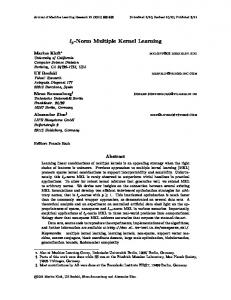
Fig. 1: Illustration of virtual labels. The base classifier f B,m is learned with the base kernel function km and the labeled training data from D, where m = 1, . . . , M . For each of the unlabeled target pattern x from DuT , we can obtain its decision value f B,m (x) from each base classifier. Then the virtual label y˜ of x is defined as the linear combination of its decision values f B,m (x)’s weighted ∑M by the coefficients dm ’s, i.e., y˜ = m=1 dm f B,m (x). flT,m = [f1T,m , . . . , fnT,m ]′ is the decision value vector of the labeled training data D from the target classifier, and T,m T,m ′ B,m B,m ′ fuT,m = [fn+1 , . . . , fn+n ] and fuB,m = [fn+1 , . . . , fn+n ] u u are the decision value vectors of the unlabeled target data DuT from the target classifier f T,m and the base classifier f B,m , respectively. While the objective function in (15) is not jointly convex with respect to the variables dm and wm , our iterative approach listed in Algorithm 1 can still reach the local minimum. We denote the objective inside {} of (15) as J(d). The dual of J(d) (see the supplementary material for the detailed derivation) can be derived by introducing the Lagrangian multipliers α and α∗ : J(d) = max

(α,α∗ )∈A

1 ∗ ˜ ˜ ′ (α−α∗ ) − ϵ1′n+nu (α+α∗ ), − (α−α∗ )′ K(α−α )−y 2 (16)

where ˜ = K

M ∑ m=1

˜ = y

M ∑ m=1

[ M 1 ∑ 2 In dm Km + dm ζ m=1 m=1 [ ] y = ∑M B,m , m=1 dm fu

˜m = dm K ˜m dm y

M ∑

1 I λ nu

] ,(17) (18)

A = {(α, α∗ )|α′ 1n+nu = α∗ ′ 1n+nu , 0n+nu ≤ α, α∗ ≤ C1n+nu } is the feasible set of the dual variables α and α∗ , and Km = [km (xi , xj )] ∈ ℜ(n+nu )×(n+nu ) is the kernel matrix of both the labeled patterns from D and unlabeled patterns from DuT . Recall that the dual form of the standard ϵ-SVR is as follows: max

(α,α∗ )∈A

1 − (α−α∗ )′ K(α−α∗ ) − y′ (α−α∗ ) − ϵ1′n+nu (α+α∗ ). 2 (19)

Surprisingly, (16) is very similar to (19) except for some minor changes, that is the kernel matrix K and ˜ and y ˜ , respectively. Therefore, (16) y are replaced by K

7

can be efficiently solved by using the state-of-the-art ˜ is SVM solver (e.g., LIBSVM [7]). The kernel matrix K similar to Automatic Relevance Determination (ARD) kernel used in Gaussian Process, and the second term in (17) is to control the noise of output. Interestingly, each ˜ in∑(18) can be considered as a of the last nu entries of y M so-called virtual label y˜ = m=1 dm f B,m (x) composed by the linear combination of the decision values from the base classifiers f B,m ’s on the unlabeled target pattern x (see Fig. 1 for illustration). With the optimal d and the dual variables α and α∗ , the target decision function can be found as: f (x) =

M ∑

′ ϕm (x) + b dm wm

m=1

=

∑

(αi − αi∗ )

i: αi −α∗ i ̸=0

M ∑

dm km (xi , x) + b.

m=1

Because of the use of the existing base classification functions, we then refer to this method as DTMKL f . 3.4 Computational Complexity of DTMKL Recall that DTMKL adopts the reduced gradient descent scheme as in [24] to iteratively update the coefficients of base kernels and learn the target classifier. For DTMKL AT, the overall optimization procedure is dominated by a series of the kernel classifier training3 . For example, at each iteration of DTMKL AT, the cost is essentially the same as the SVM training. Empirically, the SVM training complexity is O(n2.3 ) [23]. And so the training cost for our proposed DTMKL AT is O(Tmax × n2.3 ), where Tmax is the number of iterations in DTMKL. As shown in Section 4.5, our DTMKL AT generally converges after less than five iterations. For DTMKL f , we use multiple base classifiers. For example, the base classifiers SVM AT can be pre-learned and adapted from the existing classifier SVM A at very little computational cost by using warm start strategy or using A-SVM. Thus, the cost of the calculation of the virtual labels for DTMKL f is not significant. Recall that DTMKL f incorporates both labeled and unlabeled patterns in the training stage. Therefore, the training complexity of DTMKL f is O(Tmax × (n + nu )2.3 ). The testing complexity of DTMKL AT and DTMKL f depends on the number of support vectors learned from the training stage. And we show in Table 3 that our methods DTMKL AT and DTMKL f take less than one minute to finish the whole prediction process for about 21,213 test samples from each of 36 concepts on the TRECVID data set, which are as fast as the MKL algorithm. 3. Here, we suppose multiple base kernels can be precomputed and loaded into memory before the DTMKL training. Then∑ the computational cost for the calculation of the learned kernel K = M m=1 dm Km which takes O(M n2 ) time can be ignored.

3.5

Discussions with Related Work

Our work is different from the prior cross-domain learning methods such as [6], [11], [15], [16], [31], [36]. These methods use standard kernel functions for SVM training, in which the kernel parameters are usually determined through cross-validation. Recall that the kernel function plays a crucial role in SVM. When the labeled data from the target domain are limited, the cross-validation approach may not choose the optimal kernel, which significantly degrades the generalization performance of SVM. Moreover, most existing cross-domain learning algorithms [11], [16], [31], [36] do not explicitly consider any specific criterion to measure the distribution mismatch of samples between different domains. As demonstrated in the previous work [12], [19], [26], [36], the auxiliary classifiers (i.e., the base classifiers trained with the data from one or multiple auxiliary domains) can be used to learn a robust target classifier. Again, there is no specific criterion used to minimize the distribution mismatch between the auxiliary and target domains in these methods. In addition, the work in [12] focuses on the setting with multiple auxiliary domains and the Domain Adaptation Machine (DAM) algorithm was specifically proposed for multiple auxiliary domain adaptation problem. The algorithm Cross-Domain Regularized Regression (CDRR) and its Incremental version Incremental CDRR (ICDRR) in [19] were specifically designed for large scale image retrieval applications. In order to achieve the real-time retrieval performance on the large image data set with about 270,000 images, a linear regression function is used as the target function in [19]. Also, in the previous work [12], [19], [26], [36], only one kernel is used in the target decision function. In contrast to these methods [11], [12], [16], [19], [26], [31], [36], DTMKL is a unified cross-domain kernel learning framework, in which the optimal kernel is learned by explicitly minimizing the distribution mismatch between the auxiliary and target domains by using both labeled and unlabeled patterns. Most importantly, many kernel learning methods (e.g., SVM, SVR, KRLS and etc) can be readily embedded into our DTMKL framework to solve cross-domain learning problems. The work most closely related to DTMKL was proposed by Pan et al. [21], in which a two-step approach is used for cross-domain learning. The first step is to learn a kernel matrix of samples using the MMD criterion, and the second step is to apply the learned kernel matrix to train an SVM classifier. DTMKL is different from [21] in the following aspects: i) A kernel matrix is learned in unsupervised setting in [21] without using any label information, which is not as effective as our semi-supervised learning method DTMKL; ii) In contrast to the two-step approach in [21], DTMKL simultaneously learns a kernel function and SVM classifier; iii) The learned kernel matrix in [21] is nonparametric, thus it cannot be applied to unseen data. Instead, DTMKL can handle any new test data; iv) The optimization problem

8

in [21] is in the form of expensive semi-definite programming (SDP) [5], the time complexity of which is O(n6.5 ). As a result, it can only handle several hundred patterns. Therefore, it cannot be applied to medium or large scale applications such as video concept detection. Another related work is Adaptive Multiple Kernel Learning (AMKL) [14], in which the target classifier is constrained as the linear combination of a set of pre-learned classifiers and the perturbation function learned by multiple kernel learning. A-MKL can be considered as an extension of DTMKL AT. In A-MKL, the unlabeled target patterns are only used to measure the distribution mismatch between the two domains in the Maximum Mean Discrepancy (MMD) criterion, which is similar as in DTMKL AT and DTMKL f . In contrast, in DTMKL f , the decision values from the pre-learned base classifiers on the unlabeled target patterns are used as virtual labels in a new regularizer (i.e., the last term in (15)) in order to enforce that the decision values from the target classifier and the existing base classifiers are similar on the unlabeled target patterns. Moreover, A-MKL classifier can also be used as one base classifier in DTMKL f . Multiple Kernel Learning (MKL) methods [18], [24], [28] also simultaneously learn the decision function and the kernel in an inductive setting. However, the default assumption of MKL is that the training data and the test data are drawn from the same domain. When the training data and the test data come from different distributions, MKL methods cannot learn the optimal kernel with the combined training data from the auxiliary and target domains. Therefore, the training data from the auxiliary domain may degrade the classification performances of MKL algorithms in the target domain. In contrast, DTMKL can utilize the patterns from both domains for better classification performances.

In this section, we evaluate our methods DTMKL AT and DTMKL f for two cross-domain learning related applications: i) video concept detection on the challenging TRECVID video corpus and ii) text classification on the 20 Newsgroups data set and the email spam data set.

cross-domain learning methods due to the large difference between TRECVID 2007 data set and TRECVID 2005 data set in terms of program structure and production values. 36 semantic concepts are chosen from the LSCOM-lite lexicon [20], a preliminary version of LSCOM, which covers 36 dominant visual concepts present in broadcast news videos, including objects, scenes, locations, people, events and programs. The 36 concepts have been manually annotated to describe the visual content of the keyframes in both TRECVID 2005 and 2007 data sets. In this work, we focus on the single auxiliary domain and single target domain setting. To evaluate the performances of all the methods, we choose one Chinese channel CCTV4 from TRECVID 2005 data set as the auxiliary domain, and use the TRECVID 2007 data set as the target domain. The auxiliary data set DA consists of all the labeled samples from the auxiliary domain (i.e., 10,896 keyframes in CCTV4 channel). We randomly select 10 positive samples per concept from the TRECVID 2007 data set as the labeled target training data set DlT . Considering that it is computationally prohibitive to compare all the methods over multiple random training and testing splits, we report results from one split. In order to facilitate other researchers to repeat the results, we have made the selected 355 positive samples5 publicly available at http://www3.ntu.edu.sg/home2007/ S080003/sampled keyframes.txt. And for each of the 36 concepts, we have 21,213 test samples on average. Three low-level global features Grid Color Moment (225 dim.), Gabor Texture (48 dim.) and Edge Direction Histogram (73 dim.) are extracted to represent the diverse content of keyframes, because of their consistent good performances reported in TRECVID [16], [36]. Moreover, the three type of global features can be efficiently extracted, and the previous work [16], [36] also shows that the cross-domain issue exists when using these global features. Yanagawa et al. have made the three types of features extracted from the keyframes of TRECVID data sets publicly available (see [35] for more details). We further concatenate the three types of features to form a 346-dimensional feature vector for each keyframe.

4.1 Descriptions of Data Sets and Features

4.1.2

4.1.1 TRECVID data set

The 20 Newsgroups data set6 is a collection of 18,774 news documents. This data set is organized in a hierarchical structure which consists of six main categories and 20 subcategories. Some of the subcategories (from

4

E XPERIMENTS

The TRECVID video corpus4 is one of the largest annotated video benchmark data sets for research purposes. The TRECVID 2005 data set contains 61,901 keyframes extracted from 108 hours of video programs from six broadcast channels (in English, Arabic and Chinese), and the TRECVID 2007 data set contains 21,532 keyframes extracted from 60 hours of news magazine, science news, documentaries and educational programming videos. As shown in [16], TRECVID data sets are challenging for 4. http://www-nlpir.nist.gov/projects/trecvid

20 Newsgroups data set

5. A large portion of keyframes in TRECVID 2007 data set have multiple labels. We therefore only have 355 unique labeled target training samples. For each concept, we make sure that there are only 10 positive samples from the target domain when training one-versus-all classifiers. It is worth noting that for some concepts (e.g., “Person”), we have fewer than 345 negative samples for model learning after excluding some training samples that are selected from other non“Person” concepts but also positively labeled as “Person”. 6. http://people.csail.mit.edu/jrennie/20Newsgroups

9

TABLE 1: Description of the 20 Newsgroups data set. Setting comp vs rec comp vs sci comp vs talk

Auxiliary Domain comp.windows.x & rec.sport.hockey comp.windows.x & sci.crypt comp.windows.x & talk.politics.mideast

the same category) are related to each other while others (from different categories) are not related, making this data set suitable to evaluate cross-domain learning algorithms. In the experiments, four largest main categories (i.e., “comp”, “rec”, “sci” and “talk”) are chosen for evaluation. Specifically, for each main category, the largest subcategory is selected as the target domain, while the second largest subcategory is chosen as the auxiliary domain. Moreover, we consider the largest category “comp” as the positive class and one of the three other categories as the negative class for each setting. Table 1 provides the detailed information of all three settings. To construct the training data set, we use all labeled samples from the auxiliary domain, as well as randomly choose m positive and m negative samples from the target domain. And the remaining samples in the target domain are considered as the test data which are also used as the unlabeled data for training. In the experiments, m is set as 0, 1, 3, 5, 7 and 10. For any given m, we randomly sample the training data from the target domain for 5 times, and report the means and the standard deviations of all methods. Moreover, the word-frequency feature is used to represent each document. 4.1.3 Email spam data set There are three email subsets (denoted by User1, User2 and User3, respectively) annotated by three different users in the email spam data set7 . The task is to classify spam and non-spam emails. Since the spam and nonspam emails in the subsets have been differentiated by different users, the data distributions of the three subsets are related but different. Each subset has 2,500 emails, in which one half of the emails are non-spam (labeled as 1) and the other half of them are spam (labeled as -1). On this data set, we consider three settings: i) User1 (auxiliary domain) & User2 (target domain); ii) User2 (auxiliary domain) & User3 (target domain) and iii) User3 (auxiliary domain) & User1 (target domain). For each setting, the training data set contains all labeled samples from the auxiliary domain as well as the labeled samples from the target domain, in which 5 positive and 5 negative samples are randomly chosen. And the remaining samples in the target domain are used as the unlabeled training data and the test data as well. We randomly sample the training data from the target domain for 5 times and report the means and the standard deviations of all methods. Again, the word-frequency feature is used to represent each document. 7. http://www.ecmlpkdd2006.org/challenge.html

4.2

Target Domain comp.sys.ibm.pc.hardware & rec.motorcycles comp.sys.ibm.pc.hardware & sci.med comp.sys.ibm.pc.hardware & talk.politics.guns

Experimental Setup

We systematically compare our proposed methods DTMKL AT and DTMKL f with the baseline SVM, and other cross-domain learning algorithms including Feature Replication (FR) [11], Adaptive SVM (A-SVM) [36], Cross-Domain SVM (CD-SVM) [16] and Kernel Mean Matching (KMM) [15]. We also report the results of the Multiple Kernel Learning (MKL) algorithm, in which the optimal kernel combination coefficients are learned by only minimizing the second part of DTMKL AT in (10) corresponding to the structural risk functional of SVM. Note that we do not compare with [21] because their work cannot cope with thousands of training and test samples. For all methods, we train one-versus-all classifiers. Note that the standard SVM can use the labeled training data set DlT from the target domain, the labeled training data set DA from the auxiliary domain, or the combined training data set DA ∪ DlT from both auxiliary and target domains. We then refer to SVM in the above three cases as SVM T, SVM A and SVM AT, respectively. We also report the results of MKL AT by employing the combined training data from two domains. The crossdomain learning methods FR, A-SVM, CD-SVM and KMM also make use of the combined training data set DA ∪ DlT for model learning. MKL AT and our DTMKL based methods can make use of multiple base kernels. For fair comparison, we use the same kernels for other methods including SVM T, SVM A, SVM AT, FR, A-SVM, CD-SVM and KMM. Specifically for each method, we train multiple classifiers using the same kernels and then equally fuse the decision values to obtain the final prediction results. Note that we make use of the unlabeled target training data from DuT in KMM and our DTMKL based methods. For KMM and DTMKL AT, the labeled and unlabeled training data are employed to measure the data distribution mismatch between two domains using the MMD criterion in (2). We additionally make use of the virtual labels for DTMKL f , which are the linear combination of the decision values from multiple base classifiers on the unlabeled training data from DuT . In this work, we employ SVM AT from multiple base kernels as the base classifiers in DTMKL f . With our experimental setting, cross validation is not suitable to automatically tune the optimal parameters for the target classifier, because we only have a limited number of labeled samples or even no labeled samples from the target domain. For the two text data sets, we vary the regularization parameter C for all methods and report the best result of each method with the optimal

10

C, where C ∈ {0.1, 0.2, 0.5, 1, 2, 5, 10, 20, 50}. We fix the regularization parameter C as the default value 1 in LIBSVM for the large TRECVID data set, because it is time-consuming to run the experiments multiple times using different C. 4.2.1 Details on the TRECVID data set 4,000 unlabeled samples from the target domain are randomly selected as the unlabeled training data set DuT for model learning in KMM and our DTMKL methods. Moreover, for DTMKL f , only the labeled and unlabeled samples DlT ∪DuT from the target domain are used as the training data. For KMM, the parameter B is empirically set as 0.99. And for our methods, the parameter θ in DTMKL AT and DTMKL f and the parameters λ, ζ in DTMKL f need to be determined beforehand. We empirically set ζ = 0.1 and θ = 10−5 . Recall that the parameter λ in DTMKL f is used to balance the costs from labeled data and unlabeled data. Considering that the total number of unlabeled target samples is roughly 10 times more than that of the labeled target samples, we fix λ = 0.1 in our experiments. Base kernels are predetermined for all methods. Specifically, we use four types of kernels: Gaussian kernel (i.e., k(xi , xj ) = exp(−γ∥xi − xj ∥2 )), Laplacian kernel √ (i.e., k(xi , xj ) = exp(− γ∥xi − xj ∥)), inverse square distance kernel (i.e., k(xi , xj ) = γ∥xi −x1 j ∥2 +1 ) and inverse 1 distance kernel (i.e., k(xi , xj ) = √γ∥xi −x ), where the j ∥+1 kernel parameter γ is set as the default value d1 = 0.0029 (d = 346 is the feature dimension) in LIBSVM. And for each type of kernels, we use 13 kernel parameters 1.2δ+3 γ, δ ∈ {−3, −2.5, . . . , 2.5, 3}. In total, we have 52 base kernels for all methods. Note that our framework can readily incorporate other methods such as FR. Therefore, we introduce another approach (referred to as DTMKL ATFR ) by replacing SVM with FR in DTMKL AT, in which we employ the kernel proposed in the FR method [11] to form the base kernels for DTMKL ATFR . For performance evaluation, we use non-interpolated Average Precision (AP) [8], [27], [34] which has been used as the official performance metric in TRECVID since 2001. AP is related to the multi-point average precision value of a precision-recall curve, and incorporates the effect of recall when AP is computed over the entire classification results. 4.2.2 Details on the 20 Newsgroups and email spam data sets On two text data sets, all the test data in the target domain are also considered as the unlabeled data in the training stage. And for our proposed method DTMKL f , the unlabeled data from the target domain as well as the labeled data from both the auxiliary and target domains are used to construct the training data set, i.e., DA ∪ DlT ∪ DuT . For DTMKL f , we set λ = 1 in the experiments, because the total number of unlabeled

Fig. 2: Per-concept APs of all the 36 concepts using different methods. The concepts are divided into three groups according to the positive frequency. Our methods achieve the best performances for the circled concepts. target samples is roughly the same with that of the labeled training samples from both domains. We consider two types of base kernels: linear kernel (i.e., k(xi , xj ) = x′i xj ) and polynomial kernel (i.e., k(xi , xj ) = (x′i xj + 1)a ), where a = 1.5, 1.6, . . . , 2.0. Then, we have totally 7 base kernels for all methods. Classification accuracy is adopted as the performance evaluation metric for text classification. 4.3

Results of Video Concept Detection

We compare our DTMKL methods with other algorithms on the challenging TRECVID data set for the video concept detection task. For each concept, we count the frequency (referred to as positive frequency) of positive samples in the auxiliary domain. According to the positive frequency, we partition all the 36 concepts into three groups (i.e., Group High, Group Med and Group Low), with 12 concepts for each group. The concepts in Group High, Group Med and Group Low are with high, moderate and low positive frequencies, respectively. And the average results of all methods are presented in Table 2, where Mean Average Precisions (MAPs) of the concepts in three groups and all 36 concepts are referred to as MAP High, MAP Med, MAP Low and MAP ALL, respectively. From Table 2, we have the following observations: 1) SVM A is much worse than SVM T according to the MAPs over all the 36 concepts, which demonstrates

11

TABLE 2: Mean average precisions (MAPs) (%) of all methods on the TRECVID data set. MAPs are from concepts of three individual groups and all 36 concepts. MAP MAP MAP MAP

High Med Low ALL

SVM T SVM A SVM AT MKL AT 39.6 39.4 44.1 42.1 12.0 9.2 12.7 11.7 15.3 2.5 14.5 14.4 22.3 17.0 23.8 22.7

FR 45.7 13.1 15.4 24.7

A-SVM CD-SVM KMM DTMKL AT DTMKL ATFR DTMKL f 45.4 43.8 44.0 45.0 46.7 46.5 13.1 12.1 12.7 12.9 13.7 15.1 15.3 14.9 14.5 14.6 15.8 16.4 24.6 23.6 23.7 24.2 25.4 26.0

that the SVM classifier learned with the training data from the auxiliary domain performs poorly on the target domain. The explanation is that the data distributions of TRECVID data sets collected in different years are quite different. It is interesting to observe that SVM AT outperforms SVM T and SVM A in terms of MAP High, but SVM T is better than SVM AT and SVM A in terms of MAP Low. The explanation is that the concepts in Group High generally have a large number of positive patterns in both auxiliary and target domains. Intuitively, when sufficient positive samples exist in both domains, the samples distribute densely in the feature space. In this case, the distributions of samples from two domains may overlap between each other [16], and thus, the data from the auxiliary domain may be helpful for video concept detection in the target domain. On the other hand, for the concepts in Group Low, the positive samples from both domains distribute sparsely in the feature space. It is more likely that there is less overlap between the data distributions of two domains. Therefore, for the concepts in Group Low, the data from the auxiliary domain may degrade the performance for video concept detection in the target domain. 2) MKL AT is worse than SVM AT. The assumption in MKL is the training data and the test data come from the same domain. When the data distributions of different domains change considerably in cross-domain learning, the optimal kernel combination coefficients may not be effectively learned by using MKL methods based on the combined data set from two domains. 3) FR and A-SVM outperform SVM AT in terms of MAPs from all the three groups, which demonstrates that the information from the auxiliary domain can be effectively used in FR and A-SVM to improve the classification performance in the target domain. We also observe that KMM and CD-SVM are slightly worse than SVM AT in terms of MAP ALL. A possible explanation is that in CD-SVM, k-nearest neighbors from the target domain are used to define the weights for the auxiliary patterns. When the total number of positive training samples in the target domain is very limited (e.g., 10 positive samples per concept in this work), the learned weights for the auxiliary patterns are not reliable, which may degrade the performance of CD-SVM. Similarly, KMM learns the weights for the auxiliary samples in an unsupervised setting without using any label information, which may not be as effective as other cross-domain learning methods (e.g., FR and A-SVM). 4) DTMKL AT is better than SVM AT and MKL AT

in terms of MAPs over all the 36 concepts. Moreover, DTMKL ATFR and DTMKL f outperform all other method in terms of MAPs from all the three groups. These results clearly demonstrate that the DTMKL methods can successfully minimize the data distribution mismatch between two domains and the structural risk functional through effective combination of multiple base kernels. DTMKL f is better than DTMKL ATFR in terms of MAP ALL, because of the additional utilization of the base classifiers. DTMKL ATFR or DTMKL f achieve the best results in 21 out of 36 concepts. In addition, some concepts enjoy large performance gains. For instance, the AP for the concept “Waterscape Waterfront” significantly increases from 20.0% (A-SVM) to 24.5% (DTMKL f ), equivalent to a 22.5% relative improvement; and the AP for the concept “Car” is improved from 11.9% (CD-SVM) to 14.3% (DTMKL f ), equivalent to a 20.2% relative improvement. Compared with the best results from the existing methods, DTMKL f (15.1%) enjoys a relative improvement 15.3% over FR and A-SVM (13.1%) in terms of MAP Med, DTMKL f (16.4%) enjoys a relative improvement 6.5% over FR (15.4%) in terms of MAP Low. Moreover, compared with FR (24.7%), ASVM (24.6%), KMM (23.7%), CD-SVM (23.6%), MKL AT (22.7%), SVM AT (23.8%) and SVM T (22.3%), the relative MAP improvements of DTMKL f (26.0%) over all the 36 concepts are 5.3%, 5.7%, 9.7%, 10.2%, 14.5%, 9.2% and 16.6%, respectively. 5) We also observe that DTMKL ATFR is slightly better than DTMKL f in terms of MAP High, possibly because the distributions of samples from two domains overlap between each other in this case. We therefore propose a simple predicting method by using DTMKL ATFR for the concepts in Group High and DTMKL f for the rest concepts in Group Med and Group Low. The MAP of the predicting method over all 36 concepts is 26.1%, with the relative improvements over FR, A-SVM, KMM, CD-SVM, MKL AT, SVM AT and SVM T as 5.7%, 6.1%, 10.1%, 10.6%, 15.0%, 9.7% and 17.0%, respectively. We additionally report the average training and testing time of all the methods for each concept in Table 3. All the experiments are performed on an IBM workstation (2.66 GHz CPU with 32 Gbyte RAM) with LIBSVM [7]. From Table 3, we observe that SVM T is quite fast, because it only utilizes the labeled training data from the target domain. We also observe that some MKL-based methods (i.e., MKL AT, DTMKL AT and DTMKL ATFR ) are much faster than the late-fusion based methods except SVM T in the training phase. For A-SVM and

12

TABLE 3: Average training (TR) and testing (TE) time (in second) comparisons of all methods on the TRECVID data set. For A-SVM and DTMKL f , the two numbers represent the average training time for the learning of the pre-learned classifiers and the learning of the target classifier. TR TE

SVM T SVM A SVM AT MKL AT 1 1576 1618 686 31 475 509 34

FR 1636 523

A-SVM CD-SVM KMM DTMKL AT DTMKL ATFR DTMKL f 1576+32 2287 4218 639 688 1618+186 511 485 508 41 43 52

TABLE 4: Means and standard deviations (%) of classification accuracies (ACC) of all methods with different number of positive and negative training samples (i.e., m) from the target domain on the 20 Newsgroups data set. Each result in the table is the best among all the results obtained by using different regularization parameters C ∈ {0.1, 0.2, 0.5, 1, 2, 5, 10, 20, 50}. The results shown in boldface are significantly better than the others, judged by the t-test with a significance level of 0.1. (a) comp vs. rec m 0 1 3 5 7 10

SVM T – 52.9±5.9 64.0±5.8 76.8±10.9 80.6±9.1 84.8±6.2

SVM A SVM AT MKL AT 89.0±0.0 – – 89.0±0.0 89.3±0.2 89.4±0.4 89.0±0.0 90.0±0.2 90.2±0.4 89.0±0.0 90.6±0.4 90.9±0.1 89.0±0.0 91.0±0.1 91.1±0.0 89.0±0.0 91.7±0.1 91.7±0.1

m 0 1 3 5 7 10

SVM T – 51.6±3.7 57.8±8.9 63.8±13.0 73.8±4.3 76.6±3.9

SVM A SVM AT MKL AT 70.7±0.0 – – 70.7±0.0 70.8±0.1 71.1±0.1 70.7±0.0 72.0±0.7 71.8±0.8 70.7±0.0 74.1±3.1 74.1±3.2 70.7±0.0 75.6±2.7 75.8±2.7 70.7±0.0 78.1±2.7 77.9±2.7

m 0 1 3 5 7 10

SVM T – 56.7±7.1 72.4±8.4 81.9±2.1 83.5±2.0 93.5±2.0

FR – 86.6±2.2 85.7±3.9 88.9±3.1 89.5±2.5 91.3±2.2

A-SVM CD-SVM KMM A-MKL DTMKL f – – 89.2±0.0 – 91.8±0.0 88.2±1.6 88.8±0.3 89.6±0.3 89.0±0.2 92.3±0.3 88.2±1.4 89.5±0.6 90.3±0.5 89.8±0.3 92.8±0.4 89.5±2.0 90.6±0.7 91.4±0.7 91.0±0.5 93.3±0.5 90.2±1.6 90.9±0.1 91.1±0.1 91.2±0.9 93.6±0.5 91.1±1.5 91.5±0.1 91.8±0.1 92.1±0.9 94.2±0.4

(b) comp vs. sci FR – 70.5±1.6 69.6±1.8 71.3±7.7 76.0±4.5 78.4±3.4

A-SVM CD-SVM KMM A-MKL DTMKL f – – 70.2±0.0 – 72.9±0.0 70.3±0.5 69.5±1.0 70.3±0.1 70.3±0.2 73.1±0.1 70.4±0.4 72.0±0.8 72.0±0.5 72.0±0.7 74.8±0.6 71.3±2.8 74.1±3.1 74.0±3.0 74.2±3.0 77.0±2.9 73.4±3.3 75.8±2.7 75.8±2.6 75.7±2.7 78.3±2.7 74.8±2.4 78.1±2.7 78.1±2.8 78.1±2.7 80.5±2.8

(c) comp vs. talk SVM A SVM AT MKL AT 92.9±0.0 – – 92.9±0.0 93.1±0.2 93.2±0.3 92.9±0.0 93.4±0.4 93.6±0.4 92.9±0.0 93.6±0.3 93.7±0.4 92.9±0.0 93.7±0.3 93.8±0.3 92.9±0.0 94.0±0.4 94.1±0.4

FR – 91.4±3.9 91.7±3.0 93.1±0.6 93.3±1.0 93.6±1.0

DTMKL f , the most time-consuming part in the training phase is from the learning of the pre-learned classifiers, while it is very fast to learn the target classifier. Moreover, all the MKL-based methods are also much faster than the late-fusion based methods except SVM T in the testing phase. On average, our DTMKL methods take less than one minute to finish the whole prediction phase for about 21,213 test samples from each concept, which is still acceptable in the real-world applications. 4.4 Results of Text Classification For the text classification task, we focus the comparisons between DTMKL f and other related methods using two text data sets. For each setting, we report the results of all methods obtained by using the training data from the auxiliary domain as well as m positive and m negative training samples randomly selected from the target domain, where we set m = 0, 1, 3, 5, 7 and 10 for the 20 Newsgroups data set and m = 5 for the email spam data set. We randomly sample the training data from the target domain for five times. In Tables 4

A-SVM CD-SVM – – 92.3±1.5 93.1±0.3 93.7±0.6 93.4±0.3 94.0±0.6 93.7±0.3 93.7±0.7 93.8±0.4 94.0±0.4 94.0±0.3

KMM 92.2±0.0 92.3±0.1 92.5±0.5 92.8±0.5 93.7±0.3 93.9±0.8

A-MKL DTMKL f – 94.3±0.0 94.3±0.1 94.6±0.2 94.4±0.3 94.9±0.2 94.4±0.2 95.0±0.3 94.5±0.2 95.1±0.3 94.6±0.4 95.2±0.4

and 5, we report the means and standard deviations of classification accuracies for all methods on the 20 Newsgroups and email spam data sets, respectively. It is worth noting that when there are no training samples from the target domain, DTMKL f can employ the base SVM classifiers learned from the auxiliary data only. But other methods like SVM T, SVM AT, MKL AT, FR, A-SVM, CD-SVM and A-MKL [14] cannot work in this case. Also note that for all methods, each result in Tables 4 and 5 is the best among all the results obtained by using different regularization parameters C ∈ {0.1, 0.2, 0.5, 1, 2, 5, 10, 20, 50}. From Tables 4 and 5, we have the following observations: 1) On both data sets, MKL AT is comparable with SVM AT, which shows that the auxiliary domain is relevant to the target domain. The performances of SVM T and SVM AT become better on the 20 Newsgroups data set, when the number of labeled positive and negative training samples (i.e., m) increases. And SVM AT outperforms SVM T and SVM A on both data sets, which demonstrates that it is beneficial to utilize the data from

13

TABLE 5: Means and standard deviations (%) of classification accuracies (ACC) of all methods with five positive and five negative training samples from the target domain on the email spam data set. Each result in the table is the best among all the results obtained by using different regularization parameters C ∈ {0.1, 0.2, 0.5, 1, 2, 5, 10, 20, 50}. The results shown in boldface are significantly better than the others, judged by the t-test with a significance level of 0.1. (a) User1 (auxiliary domain) & User2 (target domain) SVM T SVM A SVM AT MKL AT FR A-SVM CD-SVM KMM A-MKL DTMKL f 80.2±3.5 96.1±0.0 96.2±0.1 96.2±0.0 92.5±2.8 95.4±0.9 96.2±0.2 96.2±0.1 96.3±0.3 96.9±0.1

ACC

(b) User2 (auxiliary domain) & User3 (target domain) ACC

SVM T SVM A SVM AT MKL AT FR A-SVM CD-SVM KMM A-MKL DTMKL f 82.0±2.6 96.9±0.0 97.0±0.1 97.0±0.1 92.1±2.4 96.0±1.3 97.0±0.1 97.0±0.1 97.3±0.0 97.7±0.1

ACC

SVM T SVM A SVM AT MKL AT FR A-SVM CD-SVM KMM A-MKL DTMKL f 79.1±1.9 91.7±0.0 91.8±0.1 91.4±0.1 91.8±2.5 92.4±1.2 91.8±0.1 91.8±0.1 92.8±0.5 94.0±0.4

(c) User3 (auxiliary domain) & User1 (target domain)

0.96 0.8 0.95

0.9

0.88

0.86

MKL_AT A−SVM CD−SVM KMM DTMKL_f

0.82

0.8

0.1

0.2

0.5

1

2

5

10

20

0.76 0.74 0.72 0.7 0.68


0.66 0.64 0.62

50

0.1

0.2

Regularization parameter C

0.82

0.92

0.9

0.88

MKL_AT A−SVM CD−SVM KMM DTMKL_f 0.1

0.2

0.5

1

2

5

10

20

50


(d) comp vs. rec (m = 10)

Classification accuracy


0.84

0.94

0.82

0.93 0.92 0.91


0.9 0.89 0.88

1

2

5

10

20

0.87

50

0.1

0.2

0.5

1

2

5

10

20

50


(b) comp vs. sci (m = 5)

0.96

0.84

0.94


(a) comp vs. rec (m = 5)

0.86

0.5

(c) comp vs. talk (m = 5) 0.96


0.8


0.84


0.78



0.92

0.78

0.76 0.74

0.72

0.94

0.92

0.9


0.88

0.86

0.7 0.1

0.2

0.5

1

2

5

10

20


(e) comp vs. sci (m = 10)

50

0.84

0.1

0.2

0.5

1

2

5

10

20

50


(f) comp vs. talk (m = 10)

Fig. 3: Performance comparisons of DTMKL f with other methods in terms of the means and standard deviations of classification accuracies on the 20 Newsgroups data set by using different regularization parameters C ∈ {0.1, 0.2, 0.5, 1, 2, 5, 10, 20, 50}. We set m = 5 (top) and m = 10 (bottom).

the auxiliary domain to improve the performance in the target domain. 2) Some cross-domain learning methods (i.e., CD-SVM and KMM) generally achieve similar performances when compared with SVM AT. The explanation is that the data distributions of two domains are quite related, making it difficult for the existing cross-domain learning methods to further improve the performances in the target domain. We also observe that A-SVM is worse than SVM AT in most settings on the two text data sets. It seems that the limited number of labeled training samples from the target domain are not sufficient to facilitate robust adaptation for A-SVM. And it is interesting to observe that FR is generally worse than SVM AT on the email spam data set in terms of the means of

classification accuracies. A possible explanation is that the kernel of FR, which is constructed based on the augmented features, is less effective on this data set. Moreover, in most cases, A-MKL [14] outperforms other methods except DTMKL f in terms of the means of classification accuracies. 3) Our proposed method DTMKL f is consistently better than all other methods in terms of the means of classification accuracies on both data sets, thanks to the explicit modeling of the data distribution mismatch as well as the successful utilization of the unlabeled data and the base classifiers. As shown in Table 4, when the number of labeled positive and negative training samples (i.e., m) from the target domain increases, DTMKL f becomes better on the 20 Newsgroups data set. Moreover, judged

14

0.775

0.935

0.93

0.925

0.92

0.77

0.765

0.76

0.755

0.915

0.75

0.91

0.745

0.1

0.2

0.5

0.8

1

λ

1.5

2

3

(a) comp vs. rec

5

10

0.96

C=2 C=5


C=2 C=5



0.94

C=2 C=5

0.955

0.95

0.945

0.94

0.935

0.1

0.2

0.5

0.8

1

λ

1.5

2

3

5

0.93

10

0.1

(b) comp vs. sci

0.2

0.5

0.8

1

λ

1.5

2

3

5

10

(c) comp vs. talk

Fig. 4: Performance (i.e., the means of classification accuracies) variation of DTMKL f with respect to the balance parameter λ ∈ [0.1, 10] on the 20 Newsgroups data set. We set the regularization parameter C = 2 and C = 5. by the t-test with a significance level of 0.1, DTMKL f is significantly better than other methods in all settings.

−3

x 10 2.425

0.03450

2.42

Recall that the parameter λ in DTMKL f balances the costs from the labeled and unlabeled samples (see (15)). In Fig. 4, we take the 20 Newsgroups data set as an example to investigate the performance variation of DTMKL f with respect to the parameter λ, in which we set m = 5 and the regularization parameter C = 2 and 5. Note the total number of labeled samples from two domains and the number of unlabeled samples from the target domain are almost the same on the 20 Newsgroups data set. From Fig. 4, we have the following observations: i) The performance of DTMKL f changes with different λ in a large range (i.e., λ ∈ [0.1, 10]); ii) When λ is quite small or quite large (i.e., the cost from labeled data or unlabeled data is more important), the performances of DTMKL f generally degrade a bit; iii) When we set λ ∈ [0.5, 1.5], DTMKL f achieves the best results and is not sensitive to the parameter λ as well. In this case, both the labeled data and the unlabeled data from the target domain can be effectively utilized to learn a robust classifier. We have similar observations on this data set when using different C and m, and on the email spam data set as well.

Objective value

We also compare our proposed method DTMKL f with the competitive methods including MKL AT, ASVM, CD-SVM and KMM by using different regularization parameters C ∈ {0.1, 0.2, 0.5, 1, 2, 5, 10, 20, 50}. The results of all methods are obtained by using m positive and m negative training samples from the target domain as well as the training data from the auxiliary domain, in which we set m = 5 and 10 for the 20 Newsgroups data set in Fig. 3. From the figure, we observe that when C becomes larger, all methods tend to have better performances. In addition, our method DTMKL f consistently outperforms other methods in terms of the means of classification accuracies. Moreover, DTMKL f is also relatively stable according to the standard deviations of classification accuracies. We have similar observations on this data set when using different m and also on the email spam data set.

Objective value

0.03445

0.03440

0.03435

2.415

2.41

2.405

2.4 0.03430 1

2

3

4

5

6

7

8

9

10

Iteration

2.395

1

2

3

4

5

6

7

8

9

10

Iteration

(a) Person

(b) Airplane

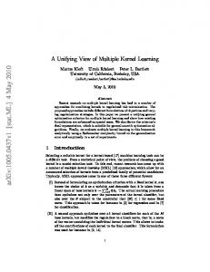
Fig. 5: Illustration of the convergence of DTMKL AT. 4.5

Convergence

In Theorem 1, we theoretically prove that DTMKL AT is jointly convex with respect to d, vm , b and ξi . Here we take two concepts “Person” and “Airplane” from the TRECVID data set as examples to experimentally demonstrate the convergence of DTMKL AT. As shown in Fig. 5, the objective values of DTMKL AT converge after less than five iterations. We have similar observations for other concepts as well.

5

C ONCLUSIONS

AND

F UTURE W ORK

In this work, we have proposed a unified cross-domain learning framework Domain Transfer Multiple Kernel Learning (DTMKL) to explore the single auxiliary domain and single target domain problem. DTMKL simultaneously learns a kernel function and a target classifier by minimizing the structural risk functional as well as the distribution mismatch between the samples from the auxiliary and target domains. By assuming that the kernel function is a linear combination of multiple base kernels, we also develop a unified learning algorithm by using the second order derivatives to accelerate the convergence of the proposed framework. Most importantly, many existing kernel methods including SVM, Support Vector Regression (SVR), Kernel Regularized Least-Squares (KRLS) and so on, can be readily incorporated into the framework of DTMKL to tackle crossdomain learning problems. Based on the DTMKL framework, we propose two methods DTMKL AT and DTMKL f by using SVM and existing classifiers, respectively. For DTMKL f , many

15

machine learning methods (e.g., SVM and SVR) can be used to learn the base classifiers. Specifically, in DTMKL f , we enforce that i) for the unlabeled target data, the target classifier produces similar decision values with those obtained from the base classifiers; ii) for the labeled target data, the decision values obtained from the target classifier are close to the true labels. Experimental results show that DTMKL f outperforms existing crossdomain learning and multiple kernel learning methods on the challenging TRECVID data set for video concept detection as well as on the 20 Newsgroups and email spam data sets for text classification. In this work, we randomly select a number of unlabeled target patterns as the training data for DTMKL f . Considering that it is beneficial to establish the optimal balance between the labeled and unlabeled patterns [10], we will investigate how to determine such optimal balance in the future. Moreover, we will also study how to automatically determine the optimal parameters for DTMKL AT and DTMKL f .

ACKNOWLEDGEMENTS This material is based upon work funded by Singapore A*STAR SERC Grant (082 101 0018) and MOE AcRF Tier1 Grant (RG15/08).

R EFERENCES [1] F. R. Bach, G. R. G. lanckriet, and M. Jordan, “Multiple Kernel Learning, Conic Duality, and the SMO Algorithm,” Proc. Int’l Conf. Machine Learning, 2004. [2] J. Blitzer, M. Dredze, and F. Pereira, “Biographies, Bollywood, Boom-boxes and Blenders: Domain Adaptation for Sentiment Classification,” Proc. Association for Computational Linguistics, pp. 440– 447, 2007. [3] A. Blum and T. Mitchell, “Combining Labeled and Unlabeled Data with Co-Training,” Proc. Annual Conference on Learning Theory, pp. 92–100, 1998. [4] K. M. Borgwardt, A. Gretton, M. J. Rasch, H.-P. Kriegel, B. ¨ Scholkopf and A. J. Smola. “Integrating Structured Biological data by Kernel Maximum Mean Discrepancy,” Bioinformatics, vol. 22, no. 4, pp. 49–57, 2006. [5] S. Boyd and L. Vandenberghe, Convex Optimization, Cambridge University Press, 2004. [6] L. Bruzzone and M. Marconcini. “Domain Adaptation Problems: a DASVM Classification Technique and a Circular validation Strategy,” IEEE Trans. Pattern Analysis and Machine Intelligence, vol. 32, no. 5, pp. 770–787, 2009. [7] C.-C. Chang and C.-J. Lin, “LIBSVM: a Library for Support Vector Machines,” Software available at http://www.csie.ntu.edu.tw/ ∼cjlin/libsvm, 2001. [8] S.-F. Chang, J. He, Y.-G. Jiang, E. E. Khoury, C.-W. Ngo, A. Yanagawa, and E. Zavesky, “Columbia University/VIREO-CityU/IRIT TRECVID2008 High-Level Feature Extraction and Interactive Video Search,” TREC Video Retrieval Evaluation Workshop (TRECVID), 2008. [9] B. Chen, W. Lam, I. W. Tsang, and T. L. Wong, “Extracting Discriminative Concepts for Domain Adaptation in Text Mining,” Proc. ACM SIGKDD Int’l Conf. Knowledge Discovery and Data Mining, pp. 179–188, 2009. [10] A. Corduneanu and T. Jaakkola, “Continuation Methods for Mixing Heterogeneous Sources,” Proc. Uncertainty in Artificial Intelligence, pp. 111–118, 2002. [11] H. Daumé III, “Frustratingly Easy Domain Adaptation,” Proc. Association for Computational Linguistics, pp. 256–263, 2007. [12] L. Duan, I. W. Tsang, D. Xu, and T.-S. Chua, “Domain Adaptation from Multiple Sources via Auxiliary Classifiers,” Proc. Int’l Conf. Machine Learning, pp. 289–296, 2009.

[13] L. Duan, I. W. Tsang, D. Xu, S. J. Maybank, “Domain Transfer SVM for Video Concept Detection,” Proc. IEEE Int’l Conf. Computer Vision and Pattern Recognition, pp. 1375–1381, 2009. [14] L. Duan, D. Xu, I. W. Tsang, J. Luo, “Visual Event Recognition in Videos by Learning from Web Data,” Proc. IEEE Int’l Conf. Computer Vision and Pattern Recognition, pp. 1959–1966, 2010. [15] J. Huang, A. J. Smola, A. Gretton, K. M. Borgwardt and B. ¨ Scholkopf, “Correcting Sample Selection Bias by Unlabeled Data,” Proc. Advances in Neural Information Processing Systems 19, pp. 601– 608, 2007. [16] W. Jiang, E. Zavesky, S.-F. Chang, and A. Loui, “Cross-Domain Learning Methods for High-Level Visual Concept Classification,” Proc. IEEE Int’l Conf. Image Processing, pp. 161–164, 2008. [17] Y.-G. Jiang, J. Wang, S.-F. Chang, and C.-W. Ngo, “Domain Adaptive Semantic Diffusion for Large Scale Context-Based Video Annotation,” Proc. IEEE Int’l Conf. Computer Vision, pp. 1420–1427, 2009. [18] G. Lanckriet, N. Cristianini, P. Bartlett, L. E. Ghaoui, and M.I. Jordan, “Learning the Kernel Matrix with Semidefinite Programming,” Journal of Machine Learning Research, vol. 5, pp. 27–72, 2004. [19] Y. Liu, D. Xu, I. W. Tsang, and J. Luo, “Textual Query of Personal Photos Facilitated by Large-Scale Web Data,” IEEE Trans. Pattern Analysis and Machine Intelligence, vol. 33, no. 5, pp. 1022–1036, 2011. [20] M. Naphade, J. R. Smith, J. Tesic, S.-F. Chang, W. Hsu, L. Kennedy, A. Hauptmann, and J. Curtis, “Large-Scale Concept Ontology for Multimedia,” IEEE MultiMedia, vol. 13, no. 3, pp. 86–91, 2006. [21] S. J. Pan, J. T. Kwok, and Q. Yang, “Transfer Learning via Dimensionality Reduction,” Proc. Assoc. for the Advancement of Artificial Intelligence, pp. 677–682, 2008. [22] S. J. Pan and Q. Yang, “A Survey on Transfer Learning,” IEEE Trans. Knowledge and Data Engineering, vol. 22, no. 10, pp. 1345–1359, 2009. [23] J. C. Platt, “Fast training of support vector machines using sequential minimal optimization,” Advances in kernel methods: support vector learning, pp. 185–208, 1999. [24] A. Rakotomamonjy, F. R. Bach, S. Canu, and Y. Grandvalet, “SimpleMKL,” Journal of Machine Learning Research, pp. 2491–2521, vol. 9, 2008. ¨ [25] B. Scholkopf and A. Smola, Learning with kernels, MIT Press, Cambridge, MA, 2002. ¨ [26] G. Schweikert, C. Widmer, B. Scholkopf, G. Rätsch, “An Empirical Analysis of Domain Adaptation Algorithms for Genomic Sequence Analysis,” Proc. Advances in Neural Information Processing Systems (NIPS), pp. 1433–1440, 2008. [27] A. F. Smeaton, P. Over, and W. Kraaij, “Evaluation Campaigns and TRECVid,” In Proc. ACM Int’l Workshop on Multimedia Information Retrieval, 2006. ¨ “Large [28] S. Sonnenburg, G. Rätsch, C. Schäfer, and B. scholkopf, Scale Multiple Kernel Learning,” Journal of Machine Learning Research, vol. 7, pp. 1531–1565, 2006. [29] A. J. Storkey and M. Sugiyama, “Mixture Regression for Covariate Shift,” Proc. Advances in Neural Information Processing Systems 19, pp. 1337–1344, 2007. [30] J. Sun, X. Wu, S. Yan, L.-F. Cheong, T.-S. Chua, and J. Li, “Hierarchical Spatio-Temporal Context Modeling for Action Recognition,” Proc. IEEE Int’l Conf. Computer Vision and Pattern Recognition, pp. 2004–2011, 2009. [31] P. Wu and T. G. Dietterich, “Improving SVM Accuracy by Training on Auxiliary Data Sources,” Proc. Int’l Conf. Machine Learning, pp. 871–878, 2004. [32] X. Wu, D. Xu, L. Duan, and J. Luo, “Action Recognition using Context and Appearance Distribution Features,” To appear in Int’l Conf. Computer Vision and Pattern Recognition, 2011. [33] A. Vedaldi, V. Gulshan, M. Varma, and A. Zisserman, “Multiple Kernels for Object Detection,” Proc. IEEE Int’l Conf. Computer Vision, pp. 606–613, 2009. [34] D. Xu and S.-F. Chang, “Video Event Recognition Using Kernel Methods with Multilevel Temporal Alignment,” IEEE Trans. Pattern Analysis and Machine Intelligence, vol. 30, no. 11, pp. 1985–1997, 2008. [35] A. Yanagawa, W. Hsu, and S.-F. Chang, “Columbia University’s Baseline Detectors for 374 LSCOM Semantic Visual Concepts,” Columbia University ADVENT Technical Report, 2007. [36] J. Yang, R. Yan, and A. G. Hauptmann, “Cross-Domain Video Concept Detection Using Adaptive SVMs,” Proc. ACM Int’l Conf. Multimedia, pp. 188–197, 2007. [37] X. Zhu, “Semi-Supervised Learning Literature Survey,” Technical report, University of Wisconsin-Madison, 2008.

16

[38] A. Zien and C. S. Ong, “Multiclass Multiple Kernel Learning,” Proc. Int’l Conf. Machine Learning, pp. 1191–1198, 2007.

Lixin Duan received the B.E. degree from the University of Science and Technology of China in 2008. He is currently pursuing the Ph.D. degree at the School of Computer Engineering, Nanyang Technological University. He was awarded the Microsoft Research Asia Fellowship in 2009, and his work won the Best Student Paper Award in CVPR 2010.

Ivor W. Tsang received the Ph.D. degree in computer science from the Hong Kong University of Science and Technology in 2007. He is currently an Assistant Professor with the School of Computer Engineering, Nanyang Technological University (NTU), Singapore. He is also the Deputy Director of the Center for Computational Intelligence, NTU. Dr. Tsang received the IEEE Transactions on Neural Networks Outstanding 2004 Paper Award in 2006, and the second class prize of the National Natural Science Award 2008, China in 2009. He was awarded the Microsoft Fellowship in 2005 and the Best Paper Award from the IEEE Hong Kong Chapter of Signal Processing Postgraduate Forum in 2006. His work was also awarded the Best Student Paper Prize at CVPR’10.

Dong Xu (M’07) received the B.E. and Ph.D. degrees from the University of Science and Technology of China, in 2001 and 2005, respectively. While pursuing his Ph.D., he was with Microsoft Research Asia, Beijing, China, and the Chinese University of Hong Kong, Shatin, Hong Kong, for more than two years. He was a Post-Doctoral Research Scientist with Columbia University, New York, NY, for one year. He is currently an Assistant Professor with Nanyang Technological University, Singapore. His current research interests include computer vision, statistical learning, and multimedia content analysis. Dr. Xu was the co-author of a paper that won the Best Student Paper Award in the prestigious IEEE International Conference on Computer Vision and Pattern Recognition in 2010.