3862
IEEE TRANSACTIONS ON NUCLEAR SCIENCE, VOL. 60, NO. 5, OCTOBER 2013
A Variable Point Kernel Dosimetry Method for Virtual Reality Simulation Applications in Nuclear Safeguards and Security Teófilo Moltó Caracena, João G. M. Gonçalves, Paolo Peerani, and Eduardo Vendrell Vidal
Abstract—This paper presents an algorithm to calculate gamma dose rates intended for virtual reality (VR) applications. It dynamically adapts the method to cope with both accuracy and time requirements. Given the real-time constraints imposed by VR applications, more accurate, but computationally intensive stochastic algorithms (e.g., Monte Carlo) are not suited to this task. On the opposite end, a Point Kernel (PK) method can be effective in some cases with as little as one point (mono PK) to define a source, in contrast with the millions of points that Monte Carlo computes. Simple mono PK codes may lack the desired accuracy in some circumstances, requiring a more detailed source representation. In this work, a novel method is presented which automatically estimates the appropriate level of detail for a source’s volumetric representation, then generates a non-regular mesh model and subsequently computes the dose rate via a PK method, performing this three-step process in real time. Index Terms—Computer simulation, gamma dosimetry, Point Kernel, virtual reality (VR).
I. INTRODUCTION IRTUAL reality (VR) has been extensively used for training simulators in many areas of research and industry. Recent developments in the fields of Nuclear Security and Safeguards [1]–[6] have shown the potential of this technology for training applications, providing advantages in terms of cost reduction and safety. The success of the VR application simulation relies greatly on its capacity to provide a real-time immersive effect to the user. In practical terms, this translates into three requirements, two of which are time-related. — First, the simulated instrument must calculate the dose rate in approximately the same amount of time as the real instrument. This time is not fixed because it depends on the type of handheld detector. Moreover, for a given detector, reading time might change depending on the energy range being measured. It typically ranges between one and five seconds.
V
Manuscript received August 09, 2012; revised December 22, 2012, May 25, 2013, and August 01, 2013; accepted August 18, 2013. Date of publication October 01, 2013; date of current version October 09, 2013. This work was supported by the European Commission’s Joint Research Centre Ph.D. grant program. T. Moltó Caracena, J. G. M. Gonçalves, and P. Peerani are with the European Commission’s Joint Research Centre, Institute for Transuranium Elements, Ispra, VA 21027 Italy (e-mail:
[email protected]). E. Vendrell Vidal is with the Universidad Politécnica de Valencia, Valencia, 46022 Spain. Color versions of one or more of the figures in this paper are available online at http://ieeexplore.ieee.org. Digital Object Identifier 10.1109/TNS.2013.2279411
— Second, the refresh rate of the visual rendering has to be as usual for VR applications about 30 frames per second (fps), in order to provide a fluid scenario movement. Furthermore, as this is a dosimetry simulation, adequate measurement accuracy is also required — Third, the deviation in dose rate computation should be in line with that of the real instruments simulated. This value is typically around 20%, which is in line with target values expected by the IAEA [7] for this kind of nondestructive analysis. Therefore the simulation is not aiming for high accuracy, but just a realistic reproduction of a handheld instrument. The first requirement limits the algorithms to those which can be run in real time, thus ruling out computationally heavy codes like Monte Carlo, despite it being optimal from the accuracy point of view, as other authors have agreed [8]–[10]. One previously explored solution to this problem is the use of a pre-calculated map of dose rates [11]. This method yields a very quick dose calculation, based on linearly interpolating doses from the nearest points in the map which come from a regular grid. The weakness of the method is that interactivity with the scenario is limited, as changes in source or shielding elements are not reflected in the dose rate and an off-line re-calculation is required. This is not compatible with the smooth interactivity one expects from a VR-based training application. In addition to stochastic methods like Monte Carlo, deterministic methods can be used to compute radiation transport. Among these, discrete ordinate methods can provide a solution for simple geometries [12] but are time consuming for the more complex geometries [13] that might arise, and are thus unsuitable for a real-time application. Alternatively, deterministic PK methods can be used [14]–[19]. These are well known in the scientific community, and in particular in the nuclear physics field. They have been developed since the 1980s to facilitate scientists’ and engineers’ calculus of gamma dose rates. Unlike methods, PK methods can cope with the requirements of this task in terms of speed and geometrical flexibility (it can work with rather complex 3-D geometries), but on the downside they do not match Monte Carlo in terms of accuracy. Nevertheless, given the large error margin conceded by the accuracy requirement, PK is suitable in the realistic case considered in this paper. We differentiate between the simpler and fast mono PK codes, like Nucleonica [14], which offer only a one point representation of the source, and the multi PK codes, which use a model source composed of a set of points called mesh. Multi PK simply multiplies the number of operations by the number
0018-9499 © 2013 IEEE
CARACENA et al.: VARIABLE POINT KERNEL DOSIMETRY METHOD FOR VIRTUAL REALITY SIMULATION APPLICATIONS
of points in the mesh. Therefore, it is obviously slower (by a factor proportional to the number of points in the mesh), but it is more accurate in cases where mono PK leads to too large a deviation, namely when the detector comes too close to the source. Many multipoint codes use a regular mesh of points to represent the source, e.g., PUTZ [15] or CIDEC [16]. These codes are aimed at shielding computations. Such applications have different requirements and execution time is not a priority. They use regular meshes with a large number of points configured offline, selecting an appropriate point density for the mesh requires users to have some knowledge of nuclear physics. These existing PK methods will be less efficient if used in VR simulations for dosimeter applications, for one or more of the following reasons. 1) Source model selection: It is not evident to a non-expert user what level of point mesh resolution is necessary. The setup of the problem should not rely on user input. It should be as automatic as possible, as agreed by [20]; 2) Dynamic variability of the model: In a VR application, the user moves freely around, and may interact with, the scenario. These changes might require variations of the source model representation, which with a VR application must be done in real-time; and 3) Efficiency of the source model: Very dense, regular, uniformly distributed point meshes guarantee accuracy at the expense of unnecessary calculations. This is the case for meshes generated by the existing software for situations where there is a large source very close to the survey meter. With this method, point density increases computational cost exponentially, hence challenging the real-time constraint. A more efficient point distribution is required to provide the required accuracy close to the source at lower computational cost. This paper presents a prototype for a VR dosimetry simulation application designed to comply with the above requirements by combining the use of the well-known PK method with novel automatic, efficient, dynamic, real-time source model representation methods. The next section explains the prototype in detail, along with the application structure, data flow and implementation aspects of the main elements: the PK dose rate computation function, the automatic resolution selector, the source model generator and the VR interface. The application was programmed using a VR-oriented software development environment, 3DVIA Virtools [21]. The prototype has been tested in order to verify the performance of the method in terms of both (a) accuracy and (b) time response. II. APPLICATION IMPLEMENTATION A. Structure of the Application The VR application is divided into two main parts: First, the dosimetry module, which implements the dose rate computation and other dosimeter-related functions. This module is executed periodically. Input data come from the current status of the relevant 3-D objects in the scenario. Outputs are the 2-D display representing the real display of the
3863
Fig. 1. DFD0: Data flow through main elements and input/output agents.
Fig. 2. DFD1 dosimetry module.
dosimeter and the 3-D rendering image of all the 3-D objects in the scenario. The second part implements the user-interfacing functions, translating input via keyboard and mouse into movement in the virtual scenario. This function updates data from the scenario’s 3-D objects, which in turn are input to the dosimetry function. The output is the rendered 3-D image of the scenario with the new positions and orientations. The following data flow diagram illustrates this scheme. B. Dosimetry Module The dosimetry module implements the three main functions of the application: Model Generator, Data Retrieval and PK Computation. These are executed sequentially in a continuous loop, together with a series of lower-priority functions. Fig. 2 shows the data-flow diagram for this module. 1) Model Generator: This module performs two tasks: testing the current model of the source and generating the new model, if necessary. It is not straightforward to assess whether a model is sufficient in terms of dose rate computation error. There are several parameters that contribute to this error and require an increase in the point resolution of the mesh. Parameters to be considered are distance (from the detector to the source), size (volume of the 3-D source) and orientation (orientation of the source with respect to the detector). In this paper, a single indicator, which can account in most cases for variations in all three parameters, is used to test the validity of the source model. This indicator, the solid angle, is
3864
IEEE TRANSACTIONS ON NUCLEAR SCIENCE, VOL. 60, NO. 5, OCTOBER 2013
Fig. 3. Variations in solid angle detect changes in distance, size, and orientation, parameters used to evaluate source model mesh validity.
defined as a measure of how large the source volume appears to an observer looking from the point where the detector is. The following figure gives 2-D examples of cases that could require a source model change. The solid angle increases when the case might require a higher point mesh resolution and is therefore a suitable parameter to evaluate the source model. A threshold value for the solid angle is set in the application, a change in the source model is triggered when that value is reached. This was empirically set to 60 . In this application, all sources are considered as parallelepipeds. This approach is valid in practical terms because many sources triggering false alarms come in this shape (e.g., a pallet stacked with chemical fertilizer sacks or a truck container full of sand). Given this representation, the Solid Angle function firstly computes the position of the eight points corresponding to the corners of the source, retrieving from the objects database the position of the barycenter, the orientation and the dimensions of the source. In the next step, it takes the position and aim direction of the detector. Then it computes the angle between the normalized vector going from the detector to the center of the source and the vector going from the detector to a corner of the source. The algorithm calculates all eight angles and keeps the two largest ones on opposite sides of the source and adds them up. Fig. 4 illustrates this process simplified to 2-D. The application compares the calculated angle with the threshold value. If the calculated angle is lower, the current model of the source is kept as it is; otherwise, the source will be passed on to the next function, Cubic Division, whereby the source is split. The cubic division method generates eight parallelepipeds from each given source in the same way that octree methods do [22], [23], i.e., creating eight new source objects which inherit the original source properties, but with sizes halved in each dimension (X,Y,Z). The newly created objects are placed evenly spaced occupying the whole volume of the original source. For each new object, the activity (A) parameter is set to an eighth of the original source activity so that the eight newly generated sources together add up to the same amount as the original source. The individual new sources can be further divided in the same iteration. This generates an irregular division of the source. Unlike uniform point meshes, this method generates a source mesh which is denser in the areas that are more significant for the
Fig. 4. Two-dimensional simplification of the solid angle calculus, addition of the largest angle on each side of the detector-to-source plane. Vertical plane running along the detector-to-source vector, which splits the eight points into two groups of four, left and right.
Fig. 5. Cubic division method simplified to 2-D. As the detector approaches the source, point resolution of the mesh is increased non-regularly.
computation. Fig. 5 shows an example of this division process simplified to 2-D. Once the solid angles of all subsource volumes have been calculated and are all under the threshold, the function stops and the model is completed for this iteration. The Model Generator phase is finished and the list of point sources updated. 2) Data Retrieval: This module has to provide all the necessary inputs for the PK Computation module. The software development environment used (3DVIA Virtools) implements a so-called 3-D object. This object type includes useful attributes like position and orientation, and is easily rendered by the Virtools engine. The object type has been extended to include attributes to be read by the Data Retrieval module which are necessary for the PK computation. These are: 1) Act: Activity of the source in Bequerels.
CARACENA et al.: VARIABLE POINT KERNEL DOSIMETRY METHOD FOR VIRTUAL REALITY SIMULATION APPLICATIONS
2) Att: Link to mass attenuation coefficient of the element tables in the PK database. 3) BUp: Link to buildup factor of the element tables in the PK database. 4) Density: Density of the element. 5) Obstacle: Faces of the geometrical model defined as obstacles for the intersection calculus. 6) Spectrum: Link to energy spectrum of the nuclide. Spectrum contains characteristic energy line and yield. The Data Retrieval module starts by collecting the spectrum and activity data from the source object attributes. It then collects the positions of the detector and the source in order to calculate the distance between them. Next, it runs the Object Intersection function, the purpose of which is to detect any obstacle between the source and detector, in order to apply the specific mass attenuation coefficient corresponding to its composition. The function is limited to one obstacle plus the self-attenuation created by the source itself. To optimize performance the self-attenuation of subsources is computed using the original source volume instead of the whole set of individual subsources. It takes as an input the group of defined obstacles in the scenario and the position of the detector and the source. Next, it starts a loop to check if a ray traced between source and detector intersects any individual obstacle, additional obstacles are neglected. If an obstacle is detected, the function takes its mass attenuation and buildup factor tables from the PK database and the density attribute of the obstacle. The thickness of the obstacle is calculated as the distance between the intersection points (entry and exit) of the ray traced through the obstacle. If no obstacle is found, air is selected as the default medium—in practical terms, an obstacle made of air, the thickness of which is the distance from the detector to the surface of the volume. The data gathered are sent to the PK Computation module. 3) PK Computation: This module performs the dose rate computation using the well-known PK method. To do so, it uses the input received from the Data Retrieval module, plus the absorption coefficient (which accounts for the energy absorbed in the detector volume). This parameter is set by default to human tissue, but can be changed to air or silicon if necessary. The PK method implemented is based on two steps. First, the radiation intensity at the point where the detector is placed (I) is computed, on the basis of initial intensity at the source and distance between the source and the detector squared (R). Secondly, the attenuation due to a possible obstacle between the source and the detector, including the source itself (self-absorption), is estimated on the basis of the following physical and chemical properties of the material: thickness (d), density and linear attenuation coefficient . The following equation relates these factors:
3865
Fig. 6. Illustration of Point Kernel scheme showing the disposition of the elements used in the calculus for (1).
the beam that is removed per unit distance in the medium as a result of three basic processes: photoelectric effect, Compton scattering and pair production, the thickness of the obstacle (length of the segment of the detector-to-source-center vector that lies within the volume of the obstacle) and the energy of the gamma beam. Also, in order to compute the dose rate received by a certain material (detector, tissue, air), a mass energy absorption coefficient is included. Finally, the algorithm takes account of the possibility that there might be more than one spectral energy line of emission, noted by the subscript ‘i’ in (2). As a result, individual energy/probability pairs have to be added. By substituting in (1) the intensity-at-source factor by source activity (A) multiplied by the energy of the gamma emission and its yield (Y) (probability of gamma emission) multiplied by mass energy absorption coefficient and the buildup factor (B), the Kerma is obtained which is equivalent to the absorbed dose (assuming charged particle equilibrium). Since the weighting factor of gamma photons is one [24], absorbed dose is substituted by equivalent dose rate, as shown in
(2) This is the equation implemented in our application for the mono PK case. Fig. 6 shows how the PK method is applied. When there is an increase in the point resolution of the source, a multi PK method is used. This alternative creates an extra loop, so for each iteration every point is treated like a new source, and the mono PK method is applied to each mesh point. Finally, the contribution of each mesh point is added up to obtain the total dose rate of the original source, as shown in Fig. 7. Starting from (2), the equation is modified by including an outer summation loop for each point (j) of the mesh, dividing total activity by the number of points in the mesh, and substituting the distance to the center of the original source (R) by each individual distance from the detector to each point (j), resulting in
(1) This implementation of the PK algorithm takes into account an estimate of dose corresponding to the photons deviated by the obstacles by introducing a buildup factor (B). This parameter is a function of the mass attenuation coefficient associated with the shielding (object) material, which is the fraction of the energy of
(3) and Buildup factors (B), mass attenuation coefficients mass absorption coefficients included in the PK database
3866
Fig. 7. Illustration of multi-PK scheme simplified to 2-D. A mesh of points represents the radiation source, in this case a 10-point mesh substitutes the single point of Fig. 6. The mono PK method is applied to each point and the individual doses added up.
are obtained by performing linear interpolation from values available from the well-known ANS data tables [25]. Energy value ranges covered in these tables are detailed in the code limitations section. If the requested values lie outside the range of energies covered by the tables, a linear extrapolation function is applied. The PK Computation implements a binary search on the data tables to find out the values for the linear interpolation for the three parameters needed. Using these three parameters and those passed on by the Data Retrieval module, the PK Computation function can finally apply the above formula to compute the equivalent dose rate in tissue (by default). The result is the equivalent dose rate in tissue expressed in mSv/h, which is made available to the interface-related modules described in the following point at a frequency which imitates the real detector’s response time. 4) Two-Dimensional Display Manager: This module includes all the functions for simulating the display of the detector. The following figure shows the data flow for this submodule, which contains five individual functions. — First, the Search Direction function simulates a visual indicator of the direction in which the source lies with respect to where the detector is. (This one of the features of the real dosimeter interface being simulated: radFINDER.) Two horizontal bars grow or shrink accordingly, indicating the angle to the source as a percentage. Each bar measures from (0%) to 90 (100%). When the source is straight ahead, both bars will be at 50%. If the angle is larger than 90 , the bars are set to zero, indicating that the source is behind the user. This function takes the information about the position and direction of the detector, and the position of the source, from the internal object database. Then, it performs a simple trigonometric computation and converts the resulting angle into a size for the horizontal bars. — Secondly, Doserate Reading is a simple function, but the most significant. It takes as an input the dose calculated by the PK Computation function in the last iteration and displays it on the screen of the 2-D dosimeter replica display. By default, it uses Sv/h as dose rate unit, but the user can switch to mRem (as used by many real instruments). — Thirdly, the Waterfall Chart function gives a visual indication of the magnitude of the last few dose readings (as represented by the vertical bars). This helps the user to locate the source, as the magnitude will be directly proportional to the distance for a given source. An increasing set
IEEE TRANSACTIONS ON NUCLEAR SCIENCE, VOL. 60, NO. 5, OCTOBER 2013
of bars corresponds to an approach to the source, while decreasing bars means the user is pulling away. The function simply stores the last ten dose rate values, which are provided by the Doserate Reading function. The values are converted to bars of proportional size. For each iteration, the bars are shifted leftward, the oldest measurement is disregarded, and the newest is placed on the far right of the display. — Fourthly, the Battery Indicator function is a simple function indicating the amount of battery lifetime left. Battery lifetime is set according to the detector manufacturer’s specifications. — Fifthly, Font Creations is an auxiliary function that creates and customizes the fonts used in the different sections of the 2-D display (Search Direction, Doserate Reading and Battery Indicator). C. Movement Module The final module of the application covers the movement of the user within the scenario. The main function waits for user input on keyboard and mouse. Mouse movement is translated into user’s viewpoint orientation change, allowing him/her to “look around” the scenario. Keyboard input translates into movement forward, back, left, and right, and rotation clockwise and counterclockwise. This configuration replicates that of other unrelated 3-D software (i.e., video games), so untrained users might find it familiar to use. An orbiting function allows the user to circle around the source without changing the distance and perceiving in real time the effect of being behind a shield or not. The current prototype uses mouse and keyboard, but other VR interfaces, like head-mounted displays, can be used in order to enhance the user’s immersive experience if necessary. Finally, a very simple hide function allows the user to hide the detector from the display to get a better view of the source. The rendering engine of Virtools converts these movements into the appropriate 3-D view. III. USER INTERFACE A dosimetry training application for a non-expert audience requires a simple interface isolating the user from the complex physics processes associated with the task. This is a feature of the prototype VR-based interface presented in this paper, where the use of the virtual instrument is clearly separated from its underlying working principle. The user is unaware of the algorithm used to simulate radiation transport, no need to characterize the radiation source is necessary by his part, a task which would require a great deal of expertise both in nuclear physics and the application configuration and problem set up. This makes this interface suitable for training applications where trainees are not assumed to have a deep understanding of radiation physics, as is the case for customs officers, border guards or emergency first responders. VR-based dosimetry applications aimed at decommissioning activities usually present an interface which focuses on planning
CARACENA et al.: VARIABLE POINT KERNEL DOSIMETRY METHOD FOR VIRTUAL REALITY SIMULATION APPLICATIONS
3867
Fig. 8. DFD2 2-D Display Manager Module.
Fig. 10. The detectors display is replicated by the application and shown on screen. The top left corner shows the battery indicator, top center the dose rate reading, below are direction indicators and at the bottom the waterfall chart.
Fig. 9. User view of the application. A cubic source in the center. The walls around it can be used to appreciate the result of the shielding (in real time) in the dose rate reading if the user walks behind them.
and showing work scenarios, therefore showing avatars representing the users, colored volumes to represent radiation and freedom of camera movement [26], [27]. The presented interface differs from these due to the different training aim (instrument usage instead of work planning). For this case the user is given a 3-D first-person view, enhanced with a 2-D replica of the detector’s display in the top left corner of the user’s screen. This feature facilitates the reading of the instrument by the user. Fig. 9 shows this view. Data on the 2-D display are updated periodically in order to replicate the typical measurement frequency of this kind of instrument. This display shows the information generated by the Doserate Reading, Waterfall Chart, Search Direction and Battery Indicator functions (see Fig. 10). The user can move around the virtual scenario by using a movement interface, which in this prototype is a simple keyboard and mouse combination but in future versions could involve more complex VR devices like head-mounted displays, while the application computes the dose rate in a manner completely hidden to the user. He/she does not need to understand
the physical models underlying the application, and this makes it suitable for non-expert users. The user may interact with some objects in the scenario, e.g., the two walls visible in Fig. 9 which as a shield. An objectsliding function prevents the user from walking through objects and a keep-on-floor function keeps the camera point of view at a constant height. The 3-D rendering of the scenario is generated by the CK2_3-D engine provided by the development software platform (3DVIA Virtools Version 5.0). Three-dimensional rendering is not covered by this study and, as it constantly takes only 0.5 ms (approx.) per frame on the tested computer (barely 1% of the limit stated in the time requirements), we will disregard its effect for evaluation purposes. IV. RESULTS Two sets of tests have been performed to validate this VR-based application. The first set tests the VR application against real measurements taken with a real gamma dosimeter in a typical nuclear security training exercise case. The second set of tests compares the VR application against other software codes for a reference nuclide case. All computer simulations were run on the same computer with the following characteristics: Intel Xeon E5640 CPU at 2.67 GHz, usable RAM 3.49 GB, NVIDIA Quadro FX 3800 graphics card, 32-bit Windows 7 OS, Virtools 5.0 SDK). A. Case 1: Fertilizer Stack ( K Source) Real Measurements The first case considers the measurement of the dose rate generated by a stack of potassium chloride (KCl) fertilizer sacks. This source is chosen as a test case because it is a typical cause of false alarms at radiation portals at international border crossings. Therefore, this is one of the sources that trainees need to learn to detect in training sessions.
3868
IEEE TRANSACTIONS ON NUCLEAR SCIENCE, VOL. 60, NO. 5, OCTOBER 2013
Fig. 11. Measurement positions for Test 1 KCl source.
Fig. 12. Dose rate comparison, real measurements vs. new (variable) and old (mono PK) simulation methods, frontal measurements.
Fig. 13. Dose rate comparison, real measurements vs. new (variable) and old (mono PK) simulation methods, above measurements.
In order to setup the test for the VR simulation, the activity of the source, the density and the geometry need to be defined. The manufacturer guarantees that over 95% of the fertilizer is KCl, therefore we assume the whole mass of 750 kg to be KCl. Taking the data mass numbers, isotopic abundance and activity of K from [28], we define the activity of the source as 12.54 MBq. To define the geometry of the source, the stack was measured and represented as a 110 cm long, 110 cm wide, and 60 cm tall parallelepiped. From this measurement, the volume ( cm ) was inferred and, given the
Fig. 14. Dose rate comparison, real measurements vs. new (variable) and old (mono PK) simulation methods, diagonal measurements.
mass stated by the manufacturer, the density was calculated (1.033g/cm ). The PK library is updated with a new table for KCl mass absorption coefficient, where all values are estimated as an average of the existing K and Cl table values. The 1460 keV energy line was considered with a yield of 10.72%. For the real measurements, a handheld gamma ion chamber survey meter is used (manufacturer: Fluke; model: Victoreen 451P). This apparatus detects gamma radiation above 25 keV, and it has a response time of between 1.8 and 5 s, depending on the operating range measured. The manufacturer states an accuracy of % of the reading between 10% and 100% of the range. Background was subtracted from the measurements taken with the survey meter—all the data in the tables are without background, as in this prototype the aim is to evaluate the method. Nevertheless, if a commercial version of the application is developed, background will be added as a constant on the basis of the scenario’s real geographical area background, plus a variable random coefficient. Measurements were taken at different positions varying distance and orientation (front, above, diagonal) of the source, and considering the origin of coordinates as its center, as shown in the next figure. The measurements in the tables are restricted to a maximum of 1 m because the dose rate values taken beyond this distance are affected by too large uncertainties. In the first place, accuracy is tested. The following two tables show the dose rate results obtained from the measurements,
3869
CARACENA et al.: VARIABLE POINT KERNEL DOSIMETRY METHOD FOR VIRTUAL REALITY SIMULATION APPLICATIONS
TABLE I REAL DETECTOR VERSUS. MONO PK SIMULATION
TABLE II REAL DETECTOR VERSUS NEW VR PROTOTYPE
Fig. 15. Original source is divided into 120 subsources (point mesh density). The four different levels of resolution, here represented in different colors to illustrate the concept. Four green 1st level subsources (coarse resolution), 24 orange second level subsources, 60 yellow third level subsources, and 32 red fourth level subsources (finest resolution).
TABLE III EXECUTION TIME
those obtained by simulating and the deviation expressed as a percentage. Table I shows the results for a mono PK (the simplest existing PK method) version of the VR application. Table II shows the dose rate results using the new variable non-regular source representation method developed in this work. The following graphs illustrate the deviation trends of the new (variable multi PK) and old (mono PK) methods with respect to the real measurements in the three testing configurations. Using this method at the closest simulating distance, the application generated a total of 120 subsources at four different levels of resolution, as Fig. 15 illustrates. Secondly, in order to test real-time behavior, execution time was measured for the variable case using functionality supplied by Virtools. There is no need to monitor the mono PK execution time, as it is constant (one point for all cases) and very fast (3 ms on the tested computer). Table III shows execution times for all positions measured, and the number of points representing the source at that measuring point for the variable non-regular method. The best case corresponds to the situation where, after checking solid angles, no new source generation is needed. The worst case corresponds to the situation where the solid
AND MESH DENSITY (NUMBER OF OF VR PROTOTYPE
POINTS)
angle check is over the limit and new source points need to be generated. From the difference between best and worst case, we can infer the time that each part of the method takes. The best case time corresponds to the time taken to make the PK calculus, and the difference between worst and best case is the time taken by the method to generate the new source model. B. Case 2: Water Cube (
Cs Source) Computer Simulations
The second test considers a gamma radiation source composed of the isotope Cs 137 diluted in water. The source is a cube with 20 cm sides. The total activity of the source is 43.53 GBq. Only the 662 KeV energy line is considered with a yield of 84.6%. Mass absorption coefficient and buildup factor for water are taken from [25], as well as the air absorption coefficient. This second test compares dose rate results for a specific setup already used as a benchmark case in previous dose rate experiments published in this journal [16].
3870
IEEE TRANSACTIONS ON NUCLEAR SCIENCE, VOL. 60, NO. 5, OCTOBER 2013
TABLE IV DOSE RATE RECEIVED AT DETECTION POINT (AIR MEDIUM) [MSV/H]
Fig. 16. Graph chart comparing the deviation of the new variable VR prototype (VR) with those for a Mono PK code (Nucleonica) and fixed Multi PK codes (CIDEC and Fixed 64).
The VR application is tested against the results provided by other PK non-VR software which the authors considered a representative selection of the state of the art of the different types of methods: one multi-PK code CIDEC (chosen as the representative of multi-PK codes because it’s performance has already been proved in a previous IEEE TNS) and a mono PK code (NUCLEONICA) chosen due to its simplicity of use and availability. MCNP was chosen because Monte Carlo methods are regarded as a valid benchmark code by all the authors referenced. The version used is MCNP Version 4C2 (simulating 10 million particles). Furthermore, in order to compare standard regularly spaced point meshes with the developed non-regular mesh representation, a fixed 64-point regular mesh version is also tested in the same configuration. Sixty-four points is chosen because this is the maximum number of mesh points the developed application uses for this case (at the shortest distance measured), so both regular and non-regular meshes have the same number of points. The results of the dose rates calculated with the different computer codes and their deviations from the benchmark code (MCNP) are shown in Table IV; MCNP statistical error is well below 1%. To better appreciate the trends of these results, the deviations are shown on the following graph (Fig. 16). At close distances (15 cm), the mono PK code (Nucleonica) results deviate excessively, showing that it is not a valid option for our purpose. As expected the fixed regular mesh examples (CIDEC and 64 point VR) are more accurate than mono PK at the extremes, but they do not provide any advantage in the intermediate cases, despite the extra computational effort.
The developed new VR non-regular version is the most accurate in all cases except the furthest distance, not only complying with requirements but also surpassing the alternatives. Finally, in order to analyze the effect of the variable method as compared with fixed mesh methods, the total amount of time for all five measurements is calculated. There is a clear proportional relationship between run time and number of points in the mesh. Two cases are considered for VR Variable code: the best-case scenario, when no change in source representation is required after the solid angle check, and the worst-case scenario, when a new source model needs to be generated for that case. V. CODE LIMITATIONS A series of limitations are present in this prototype application. 1) Geometrical limitations: Geometrical source shapes are currently restricted to parallelepipeds. In practice, this might not be a limitation, as many cases are actually parallelepipeds (as shown in the result cases), but it can be a source of error when trying to measure large cylindrical, spherical or strongly elongated (e.g., pipes) sources at close distances. 2) Inherent PK method limitations: — First, the PK method uses a series of data tables that cover the [0.010 MeV 30 MeV] energy range for attenuation coefficients, [0.015 MeV 15 MeV] for buildup factor coefficients, and [0.01 MeV 20 MeV] for absorption coefficients. For energy lines outside the range of the tables, extrapolation is used instead of linear interpolation. In practice, this is hardly a limitation, as the apparatus being simulated have an operating range which is within the range of the application’s tables (i.e., the Victoreen detector used in testing has an energy range of [0.023 MeV 1.3 MeV]). — Secondly, another limitation of the PK method is the number of materials for which data exist. For compound materials (like Case 1- KCl), new PK coefficient tables need to be created, based on averaging mass composition of the elements contained for which data are available, possibly incurring an error. 3) Shielding limitations: Only one layer of shielding is currently considered, plus the inherent shielding (self-absorption) created by the source volume itself. In case two or more obstacles are present between the source and detector only the closest to the detector is computed. Shielding data are available only for the restricted list of materials covered by the tables.
CARACENA et al.: VARIABLE POINT KERNEL DOSIMETRY METHOD FOR VIRTUAL REALITY SIMULATION APPLICATIONS
TABLE V EXECUTION TIME CASE 2
4) Flux limitation: Only direct and buildup flux is considered; backscattering and other secondary sources are disregarded. VI. CONCLUSION A method has been developed for estimating dose rates generated by gamma sources using the point kernel method. It uses a novel approach to handle a variable source representation in real time. This method has been used to develop a prototype VR-based simulator application for training purposes. The method has been tested by comparing it with a real detector and with other existing commercial software codes. Three questions arise when trying to reach a conclusion. — First: Is this a valid method for simulating a handheld detector? The results show that the developed method can simulate the performance of handheld detectors up to IAEA accuracy requirement standards. Furthermore, it represents an improvement in terms of accuracy as compared with the previously used mono PK methods. In terms of execution time, even the worst-case measurement (0.31 s) remains well below the specified response time (1.8 s) of the detector. Therefore, the method fulfills the requirements and the answer to this question is affirmative. — Secondly: Is this detailed source representation necessary? The results from Table I show that the simpler mono PK approach, although very fast (3 ms), fails to comply with accuracy requirements; in the worst-case scenario, it produces over four times as much (89%) deviation as the limit stated in the requirement. This shows the need for a more detailed (multipoint) source representation than simple point kernel for this kind of simulation. — Thirdly: Is the developed source representation (variable non-regular) better than the existing (fixed mesh) representations? Again, the answer is ‘”yes.” The graph in Fig. 13 indicates that the developed method results in a lower deviation than a regular mesh (for the same number of points) in all measurements but one. Furthermore, the developed method provides a total execution time advantage as compared with the fixed regular mesh, as shown in Table V. REFERENCES [1] F. Vermeersch and C. Van Bosstraeten, “Development of the VISIPLAN ALARA planning tool,” in Proc. Int. Conf. Topical Issues in Nuclear Radiation and Radioactive Waste Safety, Vienna, Austria, Aug. 31–Sep. 4 31, 1998.
3871
[2] F. Vermeersch, “Dose assessment and dose optimization in decommissioning using VISIPLAN 3D ALARA planning tool,” presented at the Radiation Protection and Decommissioning Conf. ABR/BVS, Brussels, Belgium, May 14, 2003. [3] I. Szöke, “New software tools for dynamic radiological characterisation and monitoring in nuclear sites,” presented at the OECD Halden Reactor Project Seminar, Studsvik, Sweden, Apr. 17-19, 2012. [4] T. Moltó Caracena, D. Brasset, E. V. Vidal, E. R. Morales, and J. G. M. Gonçalves, “A design and simulation tool for nuclear safeguards surveillance systems,” presented at the ESARDA 31st Annu. Meeting, 2009. [5] T. M. Caracena, J. G. M. Gonçalves, P. Peerani, and E. V. Vidal, “Virtual reality based simulator for dose rate calculations in nuclear safeguards and security,” presented at the ESARDA Symp., Budapest, Hungary, 2011. [6] S. Stansfield, Application of virtual reality to nuclear safeguards and nonproliferation Sandia Nat. Lab., Albuquerque, NM, USA, 1996. [7] IAEA, International Target Values 2010 for Measurement Uncertainties in Safeguarding Nuclear Materials Int. Atomic Energy Agency, Dept. of Safeguards, Vienna, Austria, STR-368, Nov. 2010. [8] L. E. Smith et al., “Coupling deterministic and Monte Carlo transport methods for the simulation of Gamma-Ray spectroscopy scenarios,” IEEE Trans. Nucl. Sci., vol. 55, no. 5, Oct. 2008. [9] G. A. Warren, L. E. Smith, M. Cooper, and W. Kaye, “Evaluation framework for search instruments,” in IEEE Nuclear Science Symp. Conf. Rec., 2005, pp. 333–337. [10] I. M. Prokhorets, S. I. Prokhorets, M. A. Khazhmuradov, E. V. Rudychev, and D. V. Fedorchenko, “Point Kernel method for radiation fields simulation,” Probl. Atom. Sci. Technol., vol. 48, p. 106, 2007. [11] A. A. C. Mol, C. A. F. Jorge, P. M. Couto, S. C. Augusto, G. G. Cunha, and L. Landau, “Virtual environments simulation for dose assessment in nuclear plants,” Progr. Nucl. Energy, vol. 51, p. 382, 2009. [12] S. M. Bowman, “SCALE 6: comprehensive nuclear safety analysis code system,” Nucl. Technol., vol. 174, no. 2, pp. 126–148, May 2011. [13] Y. Wu et al., “CAD-based interface programs for fusion neutron transport simulation,” Fusion Eng. Design, vol. 84, no. 7-11, pp. 1987–1992, Jun. 2009. [14] “Nucleonica web-driven nuclear science;,” Dosimetry and Shielding Module 2007–11 [Online]. Available: http://www.nucleonica.net [15] D. T. Ingersoll, PUTZ: A point-kernel photon shielding code Oak. Ridge Nat. Lab., Oak Ridge, TN, USA, ORNL/TM-9803, 1986. [16] O. Vela, E. De Burgos, and J. M. Perez, “Dose rate assessment in complex geometries,” IEEE Trans. Nucl. Sci., vol. 53, no. 1, Feb. 2006. [17] S. Chucas and I. Curl, “Streaming calculations using the point-kernel code RANKERN,” in J. Nucl. Sci. Technol., Proc. 9th Int. Conf. Radiation Shielding (ICRS-9), Oct. 17–22, 1999. [18] Grove Software, Microshield 9.05 2012. [19] L. Bindel, L. Clouet, E. Castanier, J. Bonnet, G. Fleury, M. Vermuse, A. Gamess, and E. Lejeune, “PERCEVAL v4.0: A new pc code for Gamma radiation studies based upon most recent development about point kernel,” in J. Nucl. Sci. Technol., Proc. 9th Int. Conf. Radiation Shielding (ICRS-9), Oct. 17–22, 1999. [20] Y. Li et al., “Benchmarking of MCAM 4.0 with the ITER 3D model,” Fusion Eng. Design, vol. 82, pp. 2861–2866, 2007. [21] “Dassault systèmes.,” 3DVIA Virtools Version 5 1999–2008. [22] G. K. Rambally and R. S. Rambally, “Octrees and their applications in image processing,” in IEEE Southeastcon Proc., 1990, pp. 1116–1120. [23] H. Samet, “Hierarchical data structures for three-dimensional data,” in From Geoscientific Map Series to Geo-Information Systems. Hannover, Germany: Schweizerbart Science, 1992, pp. 45–58. [24] P. Grande and M. C. O’Riordan, chairmen, “Data for protection against ionizing radiation from external sources: Supplement to ICRP Publication 15,” in ICRP-21, Int. Commiss. Radiological Protection. New York: Pergamon, Apr. 1971, ICRP Committee 3 Task Group. [25] Gamma-Ray Attenuation Coefficients and Buildup Factors for Engineering Materials, ANSI/ANS-6.4.3-1991, Amer. Nat. Standards Int., New York, 1991. [26] G. Rindahl and N. K. F. Mark, “VRDose and emerging 3D software solutions to support decommissioning activities: Experiences and expectations from development and deployment of innovative technology.,” Innovative and Adaptive Technologies in Decommissioning of Nuclear Facilities (IAEA-TECDOC-1602) pp. 147–158, 2008. [27] Hale et al., “3D radiation exposure modeling tool for ALARA planning,” 2011. [28] S. Bin Samat, S. Green, and A. H. Beddoe, “The 40 K activity of one gram of potassium,” Phys. Med. Biol., vol. 42, pp. 407–413, 1997.