ICCAD’17, Hammamet - Tunisia, January 19-21, 2017
Online Process monitoring based on Kernel method Radhia. Fezai*, Ines. Jaffel* , Okba. Taouali* , Mohamed. Faouzi Harkat**, Nasreddine. Bouguila* * Laboratory of Automatic Signal and Image Processing(LARATSI), National School of Engineers of Monastir, University of Monastir, Tunisia(e-mail:
[email protected];
[email protected];
[email protected];
[email protected]) **Badji Mokthar, Anaba University, Algeria (e-mail:
[email protected]) Abstract— This paper discusses the monitoring of dynamic process. In recent years, Kernel Principal component analysis (KPCA) has gained significant attention as a monitoring method of nonlinear systems. However, the fixed KPCA model limit its application for dynamic systems. For this purpose a new Variable Moving Window Kernel PCA (VMWKPCA) method is introduced to update the KPCA model. The basic idea of this technique is to vary the size of the moving window depending on the normal change of the process. Then the VMWKPCA method is performed for monitoring a Chemical reactor (CSTR). The simulation results proved that the new method is effective. Keywords— Principal Component Analysis, Kernel principal component analysis, MWKPCA, VMWKPCA, fault detection, SPE,
T2. I.
Introduction
The demand for safe operation and product quality in the industry has pushed research to develop fault detection methods. Multivariate statistical methods like Principal Component Analysis (PCA) [1,2] partial least square [3,4]and recently independent component analysis[5,6] have been used for process monitoring. PCA is considered one of the most popular mothods for its simplicity. However, PCA method assume that the relationships between variable are linear, which limit their application if these relationships are nonlinear. To over come the problem caused by nonlinear data, Scholkopf [7] proposed in recent years a nonlinear PCA method, called kernel PCA (KPCA). KPCA can efficiently determine Principal Components(PCs) in hyper dimensional feature spaces H by means of integral operators and nonlinear kernel functions. The main idea of the KPCA approach is to first map the orignal data space into a feature space using a nonlinear function and then compute the PCs in the feature space. The principal advantages of KPCA is solving the eigenvalue problem without nonlinear optimization [8]. However, a KPCA monitoring model needs the determination of the kernel matrix, whose dimension is defined by the number of observations. Besides, the KPCA with fixed model can lead to numerous error because of the variation of parameters with the operation of the system [9,10]. The old samples are not
978-1-5090-5987-4/17/$31.00 ©2017 IEEE
representative of the current process status so that the adaptation of KPCA method is impoartant. A moving window KPCA method was developed [11] to avoid this problem and to update the KPCA model using a constant moving window size [10,11]. Choosing an appropriate moving window size is an important issue. In this paper, we propose a variable moving window KPCA (VMWKPCA) method. In this method the size of the moving window change depending on the variation of the normal process. The performance of the proposed method is proved through a simulation study. This paper is organised as follows: In Section 2, an overview of KPCA method is detailled. Then in Section 3, the identification of the KPCA model is discussed. In Section 4, the MWKPCA method is detailed and the proposed variable moving window KPCA method is described. The fault detection indices as squared prediction error (SPE) and 2 in the extended feature space and its Hotelling's T corresponding control limits are given in section 5. The simulation results using the CSTR process are presented in section 6. Finally, conclusion is given in section 7. II.
Kernel principal component analysis (KPCA)
Since basic PCA performs only on linear processes, a nonlinear PCA approach for estimating nonlinear problems, named kernel PCA was proposed in recent years [7]. The basic idea of KPCA is first to map samples from their input space to a hyper dimensional feature space via nonlinear m
function φ : → H , and then to apply a linear PCA in H. Let x1 , x2 ,..., x N ∈
m
be the N training samples, with m is
the number of variables. The covariance matrix can be written in H by the following relation : 1 N (1) C = (φ ( xi ))(φ ( xi ))T N i =1 It is supposed that φ ( xi ) , i=1,…N is mean centered and variance scaled. The principal components are calculated by solving the eigenvalue problem :
236
μV = CV =
1
N
(< (φ ( xi ), V ) >φ ( xi )
(2)
N i =1 Where < x , y > is the dot product between x and y, and μ ,V are respectively the eigenvalues and eigenvectors of the covariance matrix C. For λ ≠ 0 , the vector V can be be regarded as a linear combination of φ ( x1 ), φ ( x2 ),..., φ ( x N ). Therefore, the vector V
corresponding vectors in H be normalized, < Vk .Vk >= 1 ,k=1,..,N . Therfore, the eigenvectors α k should be normalized
< α k .α k >= 1/ λk . The kth projection of φ ( x ) into the eigenvectors Vk in the
to verify
feature space H is expressed as: N
tk =< Vk , φ ( x ) >= α ki < φ ( xi ),φ ( x ) >
can be expressed by:
i =1
N
V = α jφ ( x j )
Then, by multiplying with φ ( xk ) from the left of the both sides in (2) we obtain: μ < (φ ( xk ), V ) >=< (φ ( xk ), CV ) > , k = 1,..., N
μ α j < (φ ( xk ), φ ( x j )) >=
N
N
(5)
N
α j ( < (φ ( xk ), φ ( xi )) > ) < φ ( xi ), φ ( x j ) > i =1
j =1
Let us define the kernel matrix T
K ∈ N × N such that [7]:
k ( xi , x j ) = φ ( xi ) φ ( x j ) < φ ( xi ), φ ( x j ) >
(6)
The sigmoid, polynomial, and radial basis kernels are they representative kernel functions. In this study, the radial basis kernel is used: k ( x, y ) = exp(
− x− y
2
)
c where ܿ is the width of the gaussian kernel. The centered matrix K can be obtained by: K = K − 1N K − K 1N + 1N K 1N
1 . . . where 1N = . . 1 .
(7)
. .
(8)
Substituting (6) into (5), we obtain: 2
K α = N μ Kα
(9)
where α = [α1 , ..., α N ] . T
The equation (9) is equivalent to the this kernel eigenvalue problem: λα = Kα with λ = N μ (10) Therefore, through (3), the kith eigenvector of the covariance matrix C in H can be written as : N
Vk = α kjφ ( x j ), j =1
Furthermore, we normalized
k = 1, ..., N
α k by
is
(11)
requiring that the
the
number
of
principal
components
(PCs), α k = [α k 1 , ..., α kN ] and k x = [ k ( x1 , x ), ..., k ( x N , x )] .
Determination the number of kernel PCs
Since the number of significant principal components can vary over time [12],So it is required to determine this number. In this paper, the cumulative percent variance (CPV) method is used for the determination of the number of PCs. The CPV is a measure of the percent variance defined by the first p PCs. p
CPV ( p ) = 100
λj
j =1 N
(13)
λj
j =1
The number of principal components is retained when CPV attained a predetermined limit (95%).
IV.
. 1 . . ∈ ℜN×N . . . 1
.
p
T
III.
N
j =1
i =1
Where
(4)
Insering (3) in (4), we get:
1
= α ki k ( xi , x ) = k xα k ; k = 1, ... p
(3)
j =1
(12)
N
Dynamic Kernel PCA
A. Moving window kernel PCA (MWKPCA) The KPCA model is updated using the moving widow method when the variation occur in the process because the old sample can not represent the actual status of the system[11]. Using the moving window method, the newest observation is added to the data matrix and the oldest data is eliminated, maintaining a fixed number of measurements in the data matrix. The description of this two step procedure are given in fig.1 using a moving window of size L :
φ ( xk0 ) 0 φ ( xk +1 ) . . . φ ( x0 ) k + L −1 L× m Matrix I
φ (x ) . . . φ ( x0 ) k + L −1 ( L −1)× m 0 k +1
Matrix II
φ ( xk0+1 ) . . . φ ( x0 ) k + L −1 φ ( x0 ) k+L L×m Matrix III
Fig. 1 Two step adaptation to form a new data window.
237
changes. So that, we should choosing an appropriate size of the moving window in the feature space. Xiao Bin [13] developed an approach to select the appropriate size of the moving window in the linear PCA. In this paper, we propose to extend this method in the feature space. The window size of the proposed method at instant k is expressed as :
The three matrices in Fig.1 illustrate the data in the precedent window (Matrix I), the result of discarding the oldest measurement in the feature space
φ ( xk0 ) (Matrix II), and the
new window of selected sample (Matrix III) performed by adding the new data φ ( xk + L ) to the matrix II. 0
The Gram matrix K is updated if a new measurement is available and for a window size L as follow:
K11 . . . . Kk+1 = . K . (k)1 K(k+1)1 .
. . K1(k) K1(k+1)
. ∈(L+1)(L+1) . K (k)(k+1) K(k+1)(k+1)
.
. .
. .
. . K(k)(k) . . K(k+1)k
K k +1 = T a
∈ b
(L +1)(L +1)
(14)
(15)
between
Mk
is the euclidean matrix norm of the two
successive
gram
matrices
Kk and Kk−1 . ΔM 0 and ΔK0 are the averages of ΔM and ΔK determined
ΔK determined by the training data. Generally,
define
Lmax = (30 80) Lth
Lmin = (4 6) Lth with LTh
1× L
and
is the threshold value of the
p + 2 pm− p 2 . 2m The main algorithmic step of the proposed VMWKPCA method is shown as follows : Step 1: Acquire training data which represents normal process operations. Initialize the value of the mean M 0 , the kernel
size window which is defined by LTh =
We note that the size of the Gam matrix K k +1 ∈
(L +1)(L +1)
,
is equal to ( L + 1) × ( L + 1) . So , we should discards the first L× L
norm of the
by the user. ΔM 0 and ΔK0 are the averages of ΔM and
And b = K kk ∈
row and colum to get K k +1 ∈
(16)
by the training data set. α , β and ξ three parameters chosen
K11 . . . K1k . . . L× L Kk = . . . ∈ , . . . K k1 . . . K kk a = K k 1 . . . K k ( k −1) ∈
ΔKk ξ ) ΔK0
difference between two successive mean vectors and M k −1 ,
ΔKk = Kk −Kk −1
where
T
ΔM0
+β
of the moving window, ΔM k = M k − M k −1 is the euclidean vector
difference
a
ΔMk
Where Lmax and Lmin are the maximum and minimum values
.
The Gram matrix is also equal to:
Kk
Lk = Lmin + (Lmax − Lmin )exp{−( α
which his size equal to
matrix K 0 , the number of PCs p and the control limit
( L × L) .
2 SPElim,0 and Tlim,0 of the monitoring indexes SPE0 and T0 .
B. Varible Moving window kernel PCA (VMWKPCA) MWPCA keeps good efficiency and precision of the model. Despite, it’s still lacking an adaptive algorithm for MWKPCA method to update the eigenvalues and eigenvectors of the gram matrix. In general, the window size must be sufficiently large to contain enough samples for process monitoring and modeling. On the contrary, a large size window leads to an important reduction in the calculative efficiency, and when the system varies rapidly, a window containing too many outdated measurements may result in the MWKPCA failing to follow exactly the process change. In addition, when we choose a small window, the data window may not properly describe the underlying relationships among the process variables, and if the size of the window is too small , this may lead to a potential danger due to the non detected abnormal
Step 2: For a new sample xk +1 , compute the kenel vector
2
kk +1 ∈ℜ1× N . Step 3: Calculate SPEk +1 and Tk2+1 . 0 Step 4: If SPEk +1 < SPElim, k or Tk2+1