{smn6,hamarneh}@sfu.ca. ABSTRACT. We propose a variational method for overlapping cervical cell segmentation in Pap smear images. Number and type of ...
A VARIATIONAL APPROACH FOR OVERLAPPING CELL SEGMENTATION Masoud S. Nosrati, Ghassan Hamarneh Medical Image Analysis Lab., Simon Fraser University, BC, Canada {smn6,hamarneh}@sfu.ca ABSTRACT We propose a variational method for overlapping cervical cell segmentation in Pap smear images. Number and type of cells (typically inferred from features such as shape and area of cytoplasm and nucleus) are two important factors in detecting pre-cancerous changes in the uterine cervix. Therefore, accurate and automatic detection and delineating of such cells are two preliminary steps toward automatic Pap smear image analysis. We evaluated our method on the dataset provided through the ISBI 2014 challenge. 1. METHODS Let Ω be a bounded subset of Rn where n is the image dimension (in this work n = 2) and I : Ω → R be a given gray-scale image. We use level sets (φ) to represents objects of interest due to its several advantages such as handling topological changes implicitly, being independent of parameterization and its suitability for data-driven applications. Each cell in cervical cytology images consists of two parts: nucleus and cytoplasm, where nucleus typically stands out with high contrast. We take advantage of this feature and use nuclei as good indicators for detecting cells. To detect nuclei, we used the popular maximally stable extremal region detector (MSER) [1]. We noticed that MSER is not able to detect all nuclei, therefore we trained a random decision forest classifier (RF) to find the most probable nuclei locations. We combined the results of two nuclei detectors and filtered out the non-elliptical connected components to obtain final nuclei candidates. We represent each cytoplasm and its corresponding nucleus by φci (x) : Ω → R and φni (x) : Ω → R as two signed distance map (SDM) functions, respectively, where φci (x) > 0 is inside and φci (x) < 0 is outside the ith cytoplasm and φci (x) = 0 on the boundary of the ith cytoplasm (similarly for φni ). We leverage several prior information and define the following energy functional
where ER is the regional term, ED is the distance prior between the boundary of the cytoplasm and its corresponding nucleus, ES is the elliptical shape prior, EO is an overlap constraint that motivates neighbouring cytoplasms to be excluded from one another (to not overlap), and R is the regularization term that ensures a smooth boundary of the segmented cells. λ1 to λ4 are positive weights balancing the contribution of each term in (1). We define the regional term ER as Z ER (φci , φni ) = ξ(x)g bg (x)H(−φci (x))dx Ω Z + ξ(x)g c (x)H(φci (x))H(−φni (x))dx Ω Z + ξ(x)g n (x)H(φni (x))dx , (2) Ω 1 1+|∇Gσ ∗I|
encourages the evolving contours to where ξ(x) = align with edges (Gσ is the Gaussian kernel with standard deviation of σ), g bg (x), g c (x) and g n (x) are the regional terms that measure the agreement of the image pixel x ∈ Ω with the background, cytoplasm and nucleus statistical models, respectively, and are calculated as follows g bg (x) = − log pbg (x|I(x)) ,
(3)
where pbg (x|I(x)) is the probability of a given pixel x belonging to background. We calculate g c (x) and g n (x) similar to (3). pbg (x|I(x)), pc (x|I(x)) and pn (x|I(x)) are estimated by training a random forest using the provided ground truth segmentation in the training set. Using the signed distance functions enables us to efficiently control the relative distance d between the boundary of the cytoplasm and its nucleus by introducing the distance term ED as Z c n ED (φi , φi ; d) = ξ(x)w(x) k φci (x) − φni (x) − d k2 dx. Ω
(4) Eq. (4) ensures that the nucleus, φni , is contained within the cytoplasm, φci , while maintaining the distance of d pixels E(φc , φn ) = λ1 ER (φci , φni ) + λ2 ED (φci , φni ) between them. w(x) is a spatially adaptive weight which i=1 i=1 N N N controls the distance prior influence. We incorporate this X XX X + λ3 ES (φci ) + λ4 EO (φci , φcj ) + R(φci , φni ) , weight as we observed large variation in the cell sizes and the distance between the nucleus and the cytoplasm. In regions i=1 i=1 j∈Ni i=1 where the density of nuclei is large the distance prior must (1) N X
N X
Table 1: Quantitative results on the training and test sets. JI: Jaccard index; TPR: True positive rate (pixel-level); FPR: False positive rate (pixel-level); FNR: False negative rate (cell/object-level). Training Set: TPR/FPR (FNR) d=DSC JI> 0.6
λ1
λ2
λ3
λ4
JI> 0.5
1 1.5
1.5 1.5
0.15 0.15
1 0.5
0.84/0.0041 (0.01) d=0.87 0.90/0.0104 (0.01) d=0.86
λ1
λ2
λ3
λ4
JI> 0.5
1 1.5
Lu et al. [2] 1.5 0.15 1.5 0.15
1 0.5
0.88/0.0032 (0.02) 0.87/0.0038 (0.01) d=0.87 0.90/0.0066 (0.01) d=0.84
0.84/0.0039 (0.01) d=0.87 0.90/0.0103 (0.01) d=0.86
JI> 0.7
JI> 0.8
0.85/0.0039 (0.03) d=0.88 0.90/0.0095 (0.04) d=0.87
0.86/0.0034 (0.14) d=0.89 0.91/0.0072 (0.21) d=0.89
Test Set: TPR/FPR (FNR) d=DSC JI> 0.6 0.89/0.0025 (0.09) 0.87/0.0036 (0.02) d=0.86 0.90/0.0060 (0.05) d=0.85
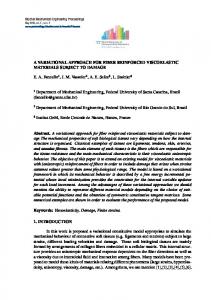
be enforced more strongly to prevent the cytoplasm’s contour from growing too far from its nucleus, while in regions with no or sparse nuclei we relax the distance prior and let the regional term dictate the contour, Fig.1. In this work we calculate w as w = eSDM (all nuclei)/20 . The shape prior term is defined as follows [2, 3] Z ES (φci ) = ξ(x)H(`(φci (x)))dx , (5) Ω
where `(φci ) returns the signed distance map of the elliptical shape approximation of φci . The fourth term in (1), EO , limits the overlapping between two neighbouring cytoplasms and penalizes the common area between two neighbouring cells and is defined as Z EO (φci , φcj ) = ξ(x)H(φci (x))H(φcj (x))dx. (6)
JI> 0.7
JI> 0.8
0.92/0.0023 (0.21) 0.87/0.0032 (0.07) d=0.87 0.90/0.0051 (0.14) d=0.87
0.93/0.0017 (0.34) 0.88/0.0024 (0.24) d=0.90 0.90/0.0033 (0.32) d=0.90
(a) (b) (c) Fig. 1: Adaptive weighted distance prior. (a) Weighting map. Segmentation (b) without and (c) with adaptive weight. nuclei detection rate with two recently proposed methods. Using non-optimized MATLAB code on a 3.4 GHz CPU with 16 GB RAM, our method segment each cell in ∼4 seconds which is ∼14 times faster than Lu et al. [2] (56 sec. per cell). Table 2: Nuclei detection results
Ω
The last term in (1) is the regularization term. Here, we adopt the total variation regularization � � Z c n c n R(φi , φi ) = ξ(x) |∇H(φi (x))| + |∇H(φi (x))| dx.
Methods Lue et al. [2] Genc¸tav et al. [5] Our method
Recall 0.90 0.93 0.98
Precision 0.69 0.74 0.99
Ω
(7) To minimize (1), we follow the approach of Chan and Vese [4] and derive the Euler-Lagrange update equation. 2. RESULTS We train our method on the training set provided by the ISBI 2014 challenge to obtain the regional models (g bg , g c and g n ) as well as weighting parameters λ1 to λ4 and evaluated the performance of our method using the provided evaluation code. The results of our method on the training and the test sets are reported in Table I (bold numbers indicates superior results). TP an FP reported in Table 1 are calculated for “well-segmented” cells (segmented cells with JI above a certain threshold). The FNR in Table 1 is due to inaccurate segmentation and/or missing cells. Note that our method has less FNR compared to [2]. In addition, Table 2 compares our
3. REFERENCES [1] J Matas et al., “Robust wide-baseline stereo from maximally stable extremal regions,” Img. vision comput., vol. 22, no. 10, pp. 761–767, 2004. [2] Z Lu et al., “Automated nucleus and cytoplasm segmentation of overlapping cervical cells,” in MICCAI, pp. 452– 460. 2013. [3] M Rousson and N Paragios, “Shape priors for level set representations,” in ECCV, pp. 78–92. 2002. [4] TF Chan and LA Vese, “Active contours without edges,” IEEE TIP, vol. 10, no. 2, pp. 266–277, 2001. [5] A Genc¸tav et al., “Unsupervised segmentation and classification of cervical cell images,” Patt. Recog., vol. 45, no. 12, pp. 4151–4168, 2012.