A Wavelet based Damage Diagnosis Algorithm Using Principal Component Analysis
K. Krishnan Nair and Anne S. Kiremidjian K. Krishnan Nair, Post Doctoral Student, Departments of Civil and Environmental Engineering & Economics Stanford University, Stanford, CA 94305. Tel.: (650) 723-6213; Fax: (650) 725-9755; Email:
[email protected] Anne S. Kiremidjian (CORRESPONDING AUTHOR) Professor, Department of Civil and Environmental Engineering, Stanford University, Stanford, CA 94305. Tel.: (650) 723-3164; Fax: (650) 723-7514; Email:
[email protected] Figures: 9 Tables: 1
1
A Wavelet based Damage Diagnosis Algorithm Using Principal Component Analysis1 K. Krishnan Nair and Anne S. Kiremidjian Department of Civil and Environmental Engineering, Stanford University, CA-94305. Email:{kknair,ask}@stanford.edu
SUMMARY Earlier papers by the authors have shown the applicability of the damage sensitive feature based on the Haar and Morlet wavelet transform of the vibration signal. In the first part of the paper, a data preprocessing algorithm is developed to compare two vibration signals which enables optimal signal selection from a database of baseline signals. The second part of the paper describes the extraction of the damage sensitive feature vector as a function of the energies at the fifth, sixth and seventh dyadic scales of the vibration signal. Both data preprocessing and feature extraction steps involve the use of principal components analysis. The process of damage detection is automated using the k-means algorithm and the Gap statistic. A simple damage extent measure is also discussed. Finally, the migration of damage sensitive feature vectors with damage is illustrated for vibration signals obtained from the ASCE Benchmark Structure. The results indicate that the developed algorithm is able to consistently detect and quantify damage for the damage patterns specified by the ASCE Benchmark Experiment. Keywords: Structural safety; Damage detection; Statistical Analysis; Signal processing; Vibration analysis.
1
This research was partially supported by the John A. Blume Doctoral Fellowship and the NSF-CMMI Grant – 0800932. The authors would also like to acknowledge the ASCE Benchmark Committee for the data and MATLAB codes. The authors would also like to thank Haeyoung Noh for providing excellent research assistance.
2
1. INTRODUCTION For early detection and assessment of structural damage, it is critical to monitor the structural response data by installing sensors on the structure under question. Wireless sensor technology has been used for this purpose and has several advantages over their wired counterparts [1, 2]. Despite its advantages, wireless sensors require low power consumption which can be achieved by embedding the damage diagnosis algorithm at the sensing unit. Thus for embedding online damage detection algorithms at the sensor level, statistical signal processing techniques along with pattern classification schemes have been used [3, 4]. These algorithms depend on features or signatures obtained from the recorded structural response signals such as acceleration, strain or other data that change with the onset of damage. Subsequently, these features are classified using pattern classification schemes. Such algorithms involve the following steps: (i) the evaluation of a structure’s operational environment which include loading conditions, temperature and humidity, (ii) the acquisition of structural response measurements and data preprocessing, (iii) the extraction of features that are sensitive to damage, and (iv) the development of statistical models for feature discrimination [3]. Previous papers by the authors have discussed the applicability of a damage sensitive feature based on the energies of the Haar and Morlet wavelet transforms of the vibration signal [5, 6]. In this paper, a damage detection algorithm based on this feature is presented. Unlike previous studies, the algorithm requires the creation of a database of normalized baseline signals and a data preprocessing algorithm is developed using principal components analysis of wavelet energies to obtain that baseline signal which is closest to the signal which is being analyzed. The damage sensitive feature is obtained by extracting the minimum variance obtained by the principal components analysis of the wavelet energies at the 5th, 6th and 7th dyadic scales. The k-means algorithm estimates the mixture centers in a dataset and the gap statistic is used to determine the optimal number of clusters in the dataset. It is hypothesized that if more than one cluster is found while comparing the damage sensitive feature of the closest baseline signal and signal being analyzed, then a change has taken place and this change is most likely due to damage.
3
This paper is organized as follows: first, a methodology is developed for selecting the signal in the database that is closest to the new signal. This selection procedure is achieved using the lower singular values of the energies of the wavelet coefficients at the first dyadic scale. Next, the damage sensitive feature vector involving the principal components analyses of the energies of the wavelet coefficients at the fifth, sixth and seventh dyadic scales is presented. Damage detection using the k-means algorithm and the gap statistic is developed in the next section. Also, a simple Euclidean metric is developed as a damage extent measure. Finally, this algorithm is tested using datasets from the ASCE Benchmark Structure [7]. 2. OVERVIEW OF ALGORITHM This algorithm requires creating a database of baseline measurements (which can include accelerations and strains) and computing the coefficients of the continuous Daubechies wavelet of order four (DB4) at appropriate scales. Baseline measurements would include vibration and strain signals obtained from the undamaged structure (at various locations) under different operational conditions such as loading and environmental conditions. The DB4 wavelet is chosen because it is similar to the Morlet wavelet. Moreover it has a discrete wavelet counterpart which makes it particularly suitable for embedding the algorithm at the sensor level. Following this, principal components analysis is performed on the energies of the DB4 wavelet coefficients at the first dyadic scale. This step helps in obtaining the closest signal in the database, which describes the loading condition of the new signal. Once the closest baseline signal in the database is chosen, feature vectors are calculated using the DB4 wavelet coefficients at the fifth, sixth and seventh dyadic scales. Intuitively, the fifth, sixth and seventh dyadic scales correspond to lower frequency modes, where in general damage is observed. This is because the data used in this paper comes from the ambient vibrations; it is unlikely that the higher modes of vibration (corresponding to lower scales) will be excited. Finally the k-means algorithm and the gap statistic are used to discriminate between damaged and undamaged states in the structure. Damage is detected when the algorithm predicts more than one cluster in the feature vectors under question. The proposed detection algorithm is as follows:
4
i
Obtain signals from an undamaged structure, from sensor i, denoted by xi(t) (i = 1,…,P), where P is the number of sensors. Divide the signal xi(t) into segments / chunks of finite duration xij(t) (j = 1,…,Q ), where Q is the number of segments. Standardize these signals to obtain a mean zero and standard deviation one signal. The database is populated with these standardized baseline signals.
ii
Compute the DB4 wavelet coefficients of the baseline signals at the first, fifth, sixth and seventh dyadic scales. Calculate the norm of the wavelet coefficients within a window size of d data points2. These are represented by
[
E baseline , j = E1,baseline , j E 5,baseline , j E 6 ,baseline , j E 7 ,baseline , j
]
∀j ∈{1,..., Q}
(1)
where Ei,baseline,j is the energy vector of the wavelet coefficients of the jth baseline signal at the ith dyadic scale. It is noted that Ei,baseline,j (i = 1, 5, 6, 7; j = 1,…,Q) is a vector of dimension int(K/d)× 1, where each baseline signal is of length K. iii
Obtain the new signal at a later time, say t. This new signal could be obtained from a potentially damaged location.
iv
Compute the DB4 wavelet coefficients of the new signals at the first, fourth, fifth and sixth dyadic scales. Energies of these coefficients are calculated in a similar fashion as performed in step ii. These are represented by
[
E new = E1, new, j E5, new, j E6, new, j E7 , new, j
]
∀j ∈{1,..., Q}
(2)
where Ei,new,j is the energy of the wavelet coefficients of the jth chunk of the new signal at the ith dyadic scale.
2
The data analyzed in this paper were stationary ambient vibration signals from the ASCE Benchmark Structure. The window size of 20 data points were chosen so that the probabilistic characteristics of the signals are preserved. In practice, the window size depends on sampling frequency and the correlation structure of the signal under question.
5
v
Selection of closest baseline signal step: Search for the best baseline signal (obtained in Step i) with similar environmental and loading conditions. This is performed as follows: •
For each baseline signal, form a matrix Z0,j = [E1,baseline,j E1,new,j] (j = 1,…,Q) of dimension int(K/d) ×2.
•
Perform a principal components (PC) analysis on Z0, j.
•
Obtain the principal direction, v1j (j = 1,…,Q). Also, obtain the minimum variance (square of the lowest singular value) and denote it as κ0j. This procedure is presented in Section 3.
•
Choose the signal closest to the new signal as that signal with the value of τj =
v11, j v 21, j
≈1 and the lowest value of κ0j, where v11,j and v21,j are the
values of the components of vector v1j. vi
Feature extraction step: Extract features by comparing the energies of the new signal with that of the best signal. This is performed as follows: •
Form a matrix Zj,k = [Ei,best,j Ei,new,j] (i = 5,6,7; j = 1,…,Q; k = 1,2,3), where Ei,best,j is the energy of the wavelet coefficients of the jth chunk of the best signal in the database at the ith dyadic scale.
•
Perform a principal component analysis on Zj,k (j = 1,…,Q; k = 1,2,3), as explained in Section 3. Obtain the minimum variance (square of the lowest singular value) and denote it as κj,k (j = 1,…,Q; k = 1,2,3).
•
Choose the damage sensitive feature vector as κ = [κ 1 κ 2 κ 3] where κ 1 is the vector whose jth component is κj,1.
vii
Classification step: Use the k-means clustering algorithm with the gap statistic to discriminate between a damaged state and an undamaged state. 6
•
Fix the number of clusters as k. For a fixed value of k, obtain the cluster centers of the grouped feature vectors X defined in Equation (3), using the k-means algorithm. κ X = undamaged κ new
(3)
where κ undamaged and κ new are the feature vectors obtained from an undamaged (the best/closest signal in the database to the new signal) and new signal respectively. Calculate the gap statistic (Tibshirani et al., 2001), as explained in Section 4. •
Use the gap statistic to determine the optimal number of clusters. If the number of clusters is greater than one, then it is hypothesized that some degree of damage has taken place. If, however, the clusters are very close based on the gap statistic, then it is concluded that there is no damage. Such signals would be stored in the baseline database.
viii
If there is damage, calculate the extent of damage by using the Euclidean distance between the means of the damaged and undamaged clusters.
ix
Go to step iii.
3. APPLICATION OF PRINCIPAL COMPONENTS ANALYSIS IN OPTIMAL SELECTION OF BASELINE SIGNAL AND FEATURE EXTRACTION Principal components analysis is used in the optimal baseline selection and in the feature extraction steps of the algorithm. In this section, the theory behind principal components is explained. Principal Components Analysis Principal components analysis (PCA) is a linear transformation used in multivariate statistical analysis in order to reduce the dimension of the dataset and to find patterns (or feature extraction) in the dataset [9]. The mathematical principle behind PCA is
7
explained as follows: Consider a centered matrix Y of dimension, say N×p. The sample covariance matrix is given by S = YTY/N-1. Then the eigen decomposition of YTY is given as Y T Y = VD 2 V T V = v 1 , v 2 ,..., v p
[
[
]
D = diag d1 , d 2 ,..., d p
]
(4)
where, V is a set of eigenvectors vi (i =1,..,p) and D is the singular value matrix. The eigenvectors vj are called the principal component directions of Y. The first principal component direction v1 has the property that z1 = Yv1 has the largest sample variance amongst all the linear combinations of the columns of Y [9]. Also, z1 is called the first principal component. In this study, principal components (PC’s) are not used as a device to reduce dimensionality but for feature extraction. This is explained in more detail in the sections below. Optimal Selection of Baseline Signal In practice, vibration data are collected under different operational conditions (loading amplitude and direction; and environmental conditions such as temperature and humidity). In order to compare ambient (or linear) vibration signals under various operational conditions, we will use the energies of the wavelet coefficients at the 1st dyadic scale to determine whether there is any difference in the loading conditions of the signal or not. While comparing a signal (from a potentially damaged location) to a baseline signal, it is assumed that damage generally occurs in the lower frequency modes, which corresponds to higher scales. Thus, lower scales are chosen for comparing loading conditions on the assumption that damage will not affect the wavelet coefficients at these scales and thus similar wavelet energies at lower scales would effectively describe the loading conditions better. Moreover the wavelet coefficients at these scales will be able to take into account the transient phenomenon such as jumps and spikes of the two signals being analyzed.
8
Figure 1 illustrates the plot of the energies of the wavelet coefficients at the first dyadic scale, for a similar and dissimilar vibration signal. The vector v1 is plotted at 45o to the x axis. In the case when we obtain acceleration datasets from similar loading conditions, it is noticed that the clouds cluster along the direction of v1. The reason for this is that these values of E1,baseline,j and E1,new,j should be similar and thus cluster around v1, implying a low variance in the direction of v2. The best signal in the database closest to the new signal is selected using the following procedure: •
Form the matrix Z0,j = [E1,baseline,j E1,new,j] ( j = 1,…,Q). Perform a principal component analysis on Z0,j. ZT0, j Z 0, j = V j D 2j V Tj
[
V j = v1 j v 2 j
[
]
D j = diag d1j , d 2j
∀j ∈{1,..., Q}
]
(4)
where, Vj is a set of eigenvectors and Dj is the singular value matrix, obtained from the decomposition of Z0,j. •
v
11, j Obtain the principal directions v1j to calculate the ratio τj = v 21, j
and
κ0, j = ( d 2j ) (j=1,…,Q). Among all the signals in the database, find that signal in 2
the database with the values of the ratio τj approximately equal to one and having the lowest value of κ0,j. In the case when the signals are not similar, the value of E1,new,1 and E1,baseline,1 would be v
11, j different and thus deviate away from the vector v1. This is measured by τj = v . If 21, j
this quantity is closer to 1 (implying that the vector v1 is at 45o to the x-axis) it would mean that the energies of the signals are similar as opposed to large value of τj. In addition, the variance (spread) in the direction v2 would give an indication of similarity. In Figure 1, a comparison of two dissimilar signals (Cluster 2) is illustrated to contrast two signals obtained from similar loading conditions (Cluster 1). To this end, the
9
principal directions will be used to obtain the directions of highest variances. The variance in the direction of the second principal direction is used to show how dissimilar the signals are. This is denoted as κ 0, whose jth component is κ0,j. Thus, the lower the value of κ0,j, the more similar the signals are. The reason why the first scale is chosen is because the coefficients at the first scale will be able to detect transient phenomenon, which is a good descriptor of loading conditions. This assumes that damage does not affect the higher frequency modes of vibration. Figure 2 illustrates the comparison of two loading conditions as defined in the ASCE Benchmark Structure Experiment. The first excitation is a series of independent filtered Gaussian white noise loads generated using a sixth - order low-pass Butterworth filter with a 100 Hz cutoff and applied at each story of the structure. The second loading is a random excitation generated by a shaker on the roof-top of the center column. Figure 2 (a) shows the histogram of τ when comparing an acceleration signal from sensor 2 for damage pattern 2 to baseline signals recorded for the same loading conditions. The values of τ are in the range of 0.8-1.6, indicating that loading conditions are similar. Also it is noted that even though damage pattern 2 is the most severe of the damage patterns, it does not affect the values of τ. Similarly, Figure 2 (b) shows the histogram of τ when comparing an acceleration signal from sensor 2 for an undamaged signal with baseline signals recorded for different loading conditions. The values of τ are much higher than one and are in the range of 4.06.0, indicating that loading conditions are not similar. Given that there is a subset of signals in the database with value of τ close to 1 (Figure 2(a)), it is necessary to identify the optimal signal in this subset closest to the new signal. This is achieved by choosing the minimum value of κ 0. Figure 3 shows the variation of κ 0 for similar loading conditions while comparing a signal from sensor 2 and damage pattern 2 to a database of eighty similar baseline signals. The lowest value of κ 0 is chosen as the best signal in the database, closest to the new signal. It should be noted that values of κ 0 is in the range of 1.8×10⁻³ to 2.5×10⁻³. Thus choosing any of these eighty baseline
10
signals would suffice for our analysis. Since the goal of this study is in automating the damage detection algorithm, we choose the optimal signal to be the one with the minimum value of κ 0. Feature Extraction In previous papers by the authors [5, 6], closed form analytical solutions of wavelet energies have been derived for single degree and multiple degree of freedom systems, thus relating it to the parameters of the structural system such as natural frequencies, damping and mode shapes. The damage sensitive feature κ is obtained by performing the principal components analysis of the wavelet energies at the 5th, 6th and 7th dyadic scales. Figure 4 illustrates the feature extraction procedure. Values of the energies of the wavelet coefficients at the fifth dyadic scale of the best baseline signal E5,best and the new signal E5,new are compared. Principal components analysis (PCA) is performed on this dataset and the variance in the second principal direction v2, denoted as κ1, is chosen as the first element of the feature vector κ. Similarly κ2 and κ3 (second and third elements of the feature vector) are derived using the energies at the sixth and seventh dyadic scales respectively. Intuitively, it can be understood that a large value of κ is a good indicator of damage. The damage sensitive features are extracted using the following procedure: •
Form a matrix Zj,k = [Ei,best,j Ei,new,j] (i = 5,6,7; j = 1,…,Q; k = 1,2,3), where Ei,best,j is the energy of the wavelet coefficients of the jth chunk of the best signal in the database at the ith dyadic scale.
•
Perform a principal component analysis on Zj,k (j = 1,…,Q; k = 1,2,3), as explained in Section 3. Obtain the minimum variance (square of the lowest singular value) and denote it as κj,k (j = 1,…,Q; k = 1,2,3).
•
Choose the damage sensitive feature vector as κ = [κ 1 κ 2 κ 3] where κ 1 is the vector whose jth component is κj,1.
It should be noted that the fifth, sixth and seventh dyadic scales are chosen by trial and error. Thus, when using this algorithm with a real structure, a finite element model of
11
the structure under question should be developed. Damage should then be induced on the finite element model and the most sensitive scales can be chosen from a similar analysis as stated in this section. In a recent study by Noh and Kiremidjian [8], the authors have found the optimal scale for feature extraction to be closely connected to the instantaneous frequency, which corresponds to that pseudo frequency at which wavelet coefficients attains a maximum value at a particular time t. In other words, the instantaneous frequency is the dominant frequency at time t. It is also shown that the instantaneous frequency is closely related to the natural frequency of the structure [8]. Figure 5 illustrates the variation of the damage sensitive feature for an undamaged case, major damage pattern 1 and minor damage pattern 6. The ASCE Benchmark experiment is described in the Appendix and in more detail in [7]. It is noted that the values of the damage sensitive feature for an undamaged case are close to zero. However, for damage patterns 1 and 6, the values of the feature vector are significantly greater than zero and form separate clouds with respect to the undamaged cloud, thus indicating damage. From Figure 5, it is also observed that as the level of damage increases the distance of the cloud from the origin increases. In the next section, a classification methodology to automate the damage detection process using the k-means algorithm and the gap statistic is explained. Also, a damage measure DM using the Euclidean distance between the means of the undamaged and damaged feature vectors is developed. 4. DAMAGE DIAGNOSIS The main premise in the developed algorithm is that there is a migration of the feature vector with the onset of damage. To automate the damage decision process, the k-means algorithm and the gap statistic are used. The k-means algorithm is a commonly used hard clustering scheme [10]. In this particular study, the k-means algorithm is used instead of Gaussian mixtures modeling [11], since there is a larger separation of clouds while using wavelet based feature vectors (Figure 5) as in comparison to the same study with the AR coefficients as feature vectors [11]. A damage measure DM using the Euclidean distance between the means of the undamaged and damaged feature vectors is also presented in this section.
12
Damage Detection using the k-means Algorithm and the Gap Statistic Figure 5 shows the results from the application of the proposed damage algorithm to the numerically simulated datasets of the ASCE Benchmark structure. From Figure 5, it can be observed that there is a distinct separation in the clouds of damage sensitive feature vector κ for damage patterns 1 and 6 with the respect to the undamaged case. The k-means algorithm is used to obtain the cluster centers with the prior assumption of the number of clusters. The gap statistic is computed to obtain the optimal number of cluster in the dataset [12]. The computation of the gap statistic is described below [12]. •
Fix the number of clusters and then use the k-means algorithm to cluster the observed data. For each of these cases, calculate Wk : k = 1,.., M, where Wk is a dispersion measure based on the within cluster distance defined in Tibshirani et al., 2001 [11].
•
Generate B reference datasets according to the uniform distribution and calculate the dispersion measure Wkb for all b = 1,…,B, and k=1,…,M.
•
Compute the mean and the standard deviation as follows µc =
1 ∑ log(Wkb ) B b 1
2 1 2 sd ( k ) = ∑ ( log(Wkb ) − µ c ) B b
s( k ) = sd 1 + •
(6)
1 B
Choose the number of clusters by using the rule given below kˆ = smallest k such that Gap ( k ) ≥ Gap (k + 1) − s k +1 Gap( k ) =
1 B ∑ log(Wkb ) − log(Wk ) B b =1
(7)
The damage detection using the k-means algorithm and the gap statistic is performed as follows: •
For k = 1 to M (M is the number of clusters)
13
o Initialize the means of the dataset to k randomly chosen points o For each cluster mean, µ j, (j= 1,…,k), find the points in the dataset closest to µ j. Denote these set of points as Cj and the number of points as nj. o Compute the new mean3 μj =
1 nj
∑x
x i ∈C j
i
(8)
where, xi is a vector belonging to cluster j, Cj. o Iterate the above two steps until convergence is obtained. o After computing the means of the dataset, the gap statistic is computed. •
Using the rules in Equation 7, find the optimal number of clusters in the dataset.
From the application of this algorithm, if the number of clusters k, is found to be greater than one, it is hypothesized that the signals come from different states of the structure and this change of state is most likely due to damage. Figure 6 illustrates the migration of clusters for an undamaged feature vector and damage pattern (DP) 6. It is observed that even though DP 6 is a minor damage pattern, there is a large separation between the feature vectors before and after damage. The kmeans algorithm is used to obtain the cluster centers in the dataset. The gap statistic predicts that there are 2 clusters in the dataset, indicating that there is damage. Figure 7 and Figure 8 illustrate a similar trend in the migration of the feature vectors for damage patterns 1-4, as defined in the ASCE Benchmark Experiment. In all these cases, the gap statistic predicts that there are two clusters in the dataset, thus 3
The dataset used for damage detection is given by the grouped feature vector X as defined in Equation 3.
14
indicating damage. The results for all sensors in the ASCE Benchmark Experiment are given in the next subsection, where the damage extent measure is developed. Damage Extent Measure The damage sensitive feature is defined as follows: DM = where,
µˆ κ,new
and
(μˆ
κ , new
T − μˆ κ,undamaged ) ( μˆ κ,new − μˆ κ,undamaged )
µˆ κ,undamaged
(9)
are the sample means of κ new and κ undamaged
respectively. Table 1 shows the variation of DM for all sensors and damage patterns as defined in the ASCE Benchmark Experiment. From Table 1, the following observations are made •
The values of DM are correlated to the amount of damage. For damage patterns 1 and 2, the values of DM are similar. A similar observation is made for damage patterns 3 and 4 for sensors placed on Faces 2 and 4 of the structure (Figure 9).
•
For minor damage patterns 3 and 6, the values of DM are high for sensors on Faces 2 and 4 in comparison to Faces 1 and 3. It is also observed that no damage is detected at sensors on Faces 1 and 3 for damage pattern 6. These are denoted as NA in Table 1. This behavior is expected since damage patterns 3 and 6 involves the reduction of stiffness of a brace on Face 2 of the ASCE Benchmark Structure (Figure 9).
•
For sensors instrumented on Faces 1 and 3 of the ASCE Benchmark Structure (Figure 9), the values of DM are significantly higher for damage pattern 4 in comparison to damage pattern 3. For example, in the case of sensor 1, the value of DM increases from 11.20 for DP 3 to 72.14 for DP 4. The reason for this trend is because DP 3 involves the removal of a brace on Face 2, whereas DP 4 is achieved by removing a brace on Face 1 and Face 2 of the structure.
15
•
All damage patterns are detected consistently using the wavelet based feature vector.
•
For all damage patterns, the values of DM are higher for sensors on Faces 2 and 4. The reason for this behavior may be attributed to the fact that this is the weak direction of the structure. CONCLUSIONS
This paper describes the development of a wavelet based damage diagnosis algorithm using principal components analysis. This algorithm requires the creation of a database of baseline measurements (which can include accelerations and strains). The first part of the paper describes a data preprocessing algorithm which enables the estimation of the optimal baseline signal closest to the new signal. Once the optimal baseline signal in the database is chosen, the damage sensitive feature vector is calculated as a function of the wavelet energies at the fifth, sixth and seventh dyadic scales. The process of damage detection is automated using the k-means algorithm and the Gap statistic. A simple damage measure based on the Euclidean distance between the means of the damaged and undamaged datasets is also described. The k-means algorithm and Gap statistic works consistently well for detecting damage patterns as defined for the ASCE Benchmark Structure. The values of DM also correlate well with the extent of damage. Although these results are promising, practical implementation of such an algorithm would require further testing and evaluation with experimental and field data. This would involve collecting structural response data under varying degrees of damage, loading conditions, environmental conditions such as temperature and humidity, as well as different sequences of damage occurrences. This would result in the creation of a larger database of baseline signals thus enabling the testing of the pre-processing, damage detection and quantification aspects of the developed algorithm. In addition, wireless sensors with this damage detection algorithm embedded on a microprocessor have to be developed and tested on experimental and real structures. It is only after extensive experimentation and field testing with calibration that these models can be widely applied. Never-the-less, the results presented here are
16
encouraging and represent a good initial step towards achieving this goal. Current research is being focused on the reliability of these algorithms for strong motion earthquake data [8, 13]. APPENDIX The ASCE Benchmark experiment is described in this appendix. The ASCE Benchmark structure is a four storey, 2 bay by 2 bay structure. The placement of the sensors and the direction of the acceleration measurements are shown in Figure 9. Damage is simulated by removal of braces thus resulting in the loss of storey stiffness and also by bolt loosening. The damage patterns include: •
Damage pattern 1: Removal of all braces on the first floor
•
Damage pattern 2: Removal of all braces on the first and third floors
•
Damage pattern 3: Removal of one brace (near sensor 2 measuring acceleration in the y-direction) on the first floor
•
Damage pattern 4: Removal of one brace on the first (near sensor 2 measuring acceleration in the y-direction) and third (near sensor 9 measuring acceleration in the x-direction) floors
•
Damage pattern 5: Damage Pattern 4 + loosening of bolts
•
Damage pattern 6: Reduction of the stiffness of a brace to 1/3rd of its original value (near sensor 2 measuring acceleration in the y-direction)
References 1. Straser, E. G. and Kiremidjian, A. S. (1998). “Modular wireless damage monitoring system for structures.”, Report No. 128, John A. Blume Earthquake Engineering Center, Department of Civil and Environmental Engineering, Stanford University, Stanford, CA. 2. Lynch, J. P., Sundararajan, A., Law, K. H., Kiremidjian, A .S. and Carryer, E. (2004). “Embedding damage detection algorithms in a wireless sensing unit for attainment of operational power efficiency.” Smart Materials and Structures, 13(4), 800-810. 3. Sohn, H., Farrar, C. R., Hunter, H. F., and Worden, K. (2001). Applying the LANL statistical pattern recognition paradigm for structural health monitoring to data from a surface-effect fast patrol boat, LANL Report LA-13761-MS, LANL Los Alamos, NM 87545.
17
4. Nair, K. K., Kiremidjian, A. S. and Law, K. H. (2006). “Time series based damage detection and localization algorithm with application to the ASCE benchmark structure.” Journal of Sound and Vibration, 291 (2), 349-368. 5. Nair, K. K. and Kiremidjian, A. S. (2009). “Damage Detection Using Haar Wavelet Transforms of Vibration Signals.” Forthcoming in ASME Journal of Applied Mechanics. 6. Nair, K. K. and Kiremidjian, A. S. (2009). “A Morlet Wavelet Based Damage Detection Algorithm.” Submitted. 7. Johnson, E. A., Lam, H. F., Katafygiotis, L. S. and Beck, J. L. (2004). “Phase I IASCASCE structural health monitoring benchmark problem using simulated data.” ASCE Journal of Engineering Mechanics, 130(1), 3-15. 8. Noh, H. and Kiremidjian, A. S. (2009). “On the use of wavelet coefficient energy for structural damage diagnosis.” 10th International Conference on Structural Safety and Reliability, Osaka, Japan. 9. Mardia, K. V., Kent, J. T. and Bibby, J. M. (2003). Multivariate Analysis, Academic Press, London. 10. Hastie, T., Tibshirani, R. and Freidman, J., (2001). Elements of Statistical Learning: Data Mining, Inference and Prediction, Springer Verlag, First edition, New York. 11. Nair, K. K. and Kiremidjian, A. S. (2007). “Time series based structural damage detection algorithm using Gaussian mixtures modeling.” ASME Journal of Dynamic Systems, Measurement and Control, 129(3), 285-293. 12. Tibshirani, R., Walther, G. and Hastie, T., 2001. “Estimating the Number of Clusters in a Dataset via the Gap Statistic,” J. of the Royal Stat. Soc: Series B, 63(2), pp. 411-423. 13. Noh, H., Nair, K. K, Lignos, D. and Kiremidjian, A. S. “On the use of wavelet based damage sensitive features for structural damage diagnosis,” Under preparation.
18
Figures
v
Cluster 2
1
E1 new,1 ,
v
2’
Similar signal
v
1’
Dissimilar signal v2
Cluster 1
E1, baseline,1
Figure 1: Illustration of a similar and dissimilar cloud by comparing E1,baseline and E1,new
19
(a)
(b)
Figure 2: Histogram of τ for sensor 2 for (a) similar loading condition with DP2 and (b) dissimilar loading conditions for undamaged cases
20
κ0
Number of records
Figure 3: Variation of κ0 for similar loading conditions comparing undamaged case and damage pattern 2
21
v1 Damaged cloud
E5, damaged
v2
κ1 = Variance in direction v2 v4
v3
Undamaged cloud
E5, best Figure 4: Illustration of damaged and undamaged cloud using principal components analysis
22
Figure 5: Variation of the damage sensitive feature vectors for damage patterns (DP) 0, 1 and 6 as defined in the ASCE Benchmark Experiment
23
(a)
(b)
Figure 6: Migration of the feature vectors κ with damage for minor patterns (a) Damage pattern 6 and (b) a zoom in of the undamaged cloud (Undamaged ο; Damaged +)
24
(a)
(b) Figure 7: Migration of the feature vectors with damage for damage patterns (a) Damage pattern 3 and (b) Damage Pattern 4 (Undamaged ο; Damaged +)
25
(a)
(b) Figure 8: Migration of the feature vectors with damage for major patterns (a) Damage pattern 1 and (b) Damage Pattern 2 (Undamaged ο; Damaged +)
26
15
14 13
16 11
10 9
12 7
6 5
8 3
2 1
4
Figure 9: Placement of sensors and directions of acceleration measurements on the ASCE Benchmark Structure [7]
27
Tables
Table 1: Variation of DM for the Morlet wavelet based damage sensitive feature for various sensors and different damage patterns
Sensor
DP1
DP2
DP3
DP4
DP5
DP6
1 2 3 4 5 6 7 8 9 10 11 12 13 14 15 16
98.07 129.31 105.89 144.37 91.81 109.14 83.77 106.05 102.21 122.73 108.8023 111.39 110.60 123.01 98.18 126.27
100.35 119.52 105.51 127.67 96.54 136.85 88.08 128.91 99.38 123.77 103.50 112.44 108.19 108.23 97.01 113.72
11.20 109.27 13.62 123.77 14.31 118.73 14.53 105.65 19.18 139.95 22.41 122.09 19.33 126.89 17.89 124.56
72.14 108.54 76.74 123.16 71.37 118.81 63.39 105.22 68.82 139.75 72.94 122.07 82.20 126.21 71.56 124.42
72.14 108.54 76.74 123.16 71.37 118.81 63.39 105.22 68.82 139.75 72.94 122.07 82.20 126.21 71.56 124.42
NA 63.36 NA 71.53 NA 79.37 NA 71.21 NA 98.04 NA 88.20 NA 83.69 NA 88.26
28