IEEE TRANSACTIONS ON ANTENNAS AND PROPAGATION, VOL. 62, NO. 5, MAY 2014
2679
A Well-Scaling Parallel Algorithm for the Computation of the Translation Operator in the MLFMA Bart Michiels, Ignace Bogaert, Member, IEEE, Jan Fostier, Member, IEEE, and Daniël De Zutter, Fellow, IEEE
Abstract—This paper investigates the parallel, distributedmemory computation of the translation operator with multipoles in the three-dimensional Multilevel Fast Multipole Algorithm (MLFMA). A baseline, communication-free parallel algorithm can compute such a translation operator in time, processes. We propose a parallel algorithm that using time. This complexity is reduces this complexity to theoretically supported and experimentally validated up to 16 384 parallel processes. For realistic cases, the implementation of the proposed algorithm proves to be up to ten times faster than the baseline algorithm. For a large-scale parallel MLFMA simulation with 4096 parallel processes, the runtime for the computation of all translation operators during the setup stage is reduced from roughly one hour to only a few minutes. Index Terms—Distributed-memory architecture, MLFMA, parallel computing, translation operator.
I. INTRODUCTION
E
LECTROMAGNETIC scattering problems involving piecewise homogeneous objects are often formulated using boundary integral equations. A method of moments (MoM) discretization then yields a dense set of linear equaunknowns. When solving this set of equations tions and iteratively, the Multilevel Fast Multipole Algorithm (MLFMA) can be used to evaluate the matrix-vector multiplication with a [1]–[3], allowing the solution complexity of only for large problems. Within the MLFMA, unknowns are hierarchically organized into an octree of boxes and interactions between these boxes are evaluated using radiation patterns and translation operators. In the three-dimensional MLFMA, the multipoles is given by [2], [3] translation operator with
(1)
Manuscript received August 06, 2013; revised November 22, 2013; accepted January 24, 2014. Date of publication February 20, 2014; date of current version May 01, 2014. The work of B. Michiels was supported by a doctoral grant from the Special Research Fund (BOF) at Ghent University. The work of I. Bogaert was supported by a post-doctoral grant from Research Foundation-Flanders (FWO-Vlaanderen). The authors are with the Department of Information Technology (INTEC), Ghent University, B-9000 Ghent, Belgium (e-mail:
[email protected]. be). Color versions of one or more of the figures in this paper are available online at http://ieeexplore.ieee.org. Digital Object Identifier 10.1109/TAP.2014.2307338
with , a vector representing the angular direction in which the translation operator is to be evaluthe translation direction ated, the wavenumber, and connecting the centers of the two interacting boxes and the Legendre polynomial and spherical Hankel function of the second kind of order respectively. Given a fixed and , the translation operator is a one-dimensional function of . multipoles In the MLFMA, translation operators with angular points. The direct calculation of a are sampled in operations. translation operator using (1) hence requires We refer to this method as the “direct method” (DM). In [4], a two-step procedure was introduced to reduce this complexity to [4], [5]. In the first step, the bandlimited function is evaluated in equidistant points in the -dimension, ranging from 0 to , using (1). In the second step, local interpopoints. Both lation is used to evaluate in the required time. This method is referred to as the “insteps require terpolation method” (IM). In this paper, we investigate an algorithm for the parallel, distributed-memory computation of the translation operator. Even though this problem is interesting in its own right, the main motivation for our work is closely related to recent advances in the development of distributed-memory, parallel algorithms for the high-frequency MLFMA [6]–[11]. State-of-the-art implementations rely on a hierarchical distribution of radiation patterns sampling points, in which radiation patterns, containing parallel processes [10]–[15]. are distributed among sampling points in This way, each process holds only local memory. Consequently, to compute the translations in the MLFMA, each process requires only a corresponding subset of the translation operator. We propose a novel algorithm based on the parallelization of the IM. The algorithm does require inter-process communication, however, the key result is that the translation opertime using parallel ator is computed in processes. For a realistic and , the proposed algorithm is roughly 10 times faster than a naive, baseline parallel algorithm. Recently, a method to compute Legendre polynomials in a , regardless of argument or degree, has been complexity of developed [16], in contrast to routines that are based on the wellknown Legendre recursion formulas. As we will explain in this paper, this is essential for our proposed algorithm to obtain a good scaling behavior. This paper is organized as follows: first, in Section II the notation is established and assumptions are stated. Section III describes the actual parallel algorithm and the computational com-
0018-926X © 2014 IEEE. Personal use is permitted, but republication/redistribution requires IEEE permission. See http://www.ieee.org/publications_standards/publications/rights/index.html for more information.
2680
IEEE TRANSACTIONS ON ANTENNAS AND PROPAGATION, VOL. 62, NO. 5, MAY 2014
TABLE I RUNTIME TO COMPUTE A TRANSLATION OPERATOR FOR AN INCREASING ( ) FOR THE DIRECT METHOD (DM), INTERPOLATION METHOD (IM), AND PARALLEL DIRECT METHOD (PDM)
plexity is derived. This theoretical work is validated by benchmarking an implementation of the algorithm in Section IV. Finally, in Section V, our conclusions are presented. II. PROBLEM DESCRIPTION AND PRELIMINARIES A. Problem Description For the high-frequency MLFMA, the required value for obtain a desired accuracy is given by [3]
to
(2) where denotes the box edge length. roughly doubles at every next level up in the MLFMA-tree. As radiation patterns and angular points, their translation operators are sampled in sampling rate increases by a factor of approximately four at each higher level. Table I lists the runtime for the sequential computation of a single translation operator using both the DM and IM and time comfor different MLFMA-levels. The plexities for the DM and IM respectively are clearly observed. In the hierarchical parallel MLFMA, the sampling points of the radiation patterns and translation operators are partitioned parallel processes in an increasing number of for every higher level in the MLFMA-tree [12], [13]. Formally angular sampling points are partitioned stated, the parallel processes, such that each process among sampling points in local memory. As both the contains problem size and the number of processes are proportionally increased with each MLFMA-level, the parallelization of the computation of the translation operator should be treated as a weak scaling parallelization problem. Therefore, the main focus of the parallelization should be the weak scaling behavior of the algorithm, rather than its strong scaling behavior, i.e., the speedup for the computation of a fixed-size translation operator as a function of the number of processes. Throughout the whole paper, the term scaling refers to weak scaling. A baseline, communication-free parallel algorithm for the distributed computation of the translation operator is easily obtained by trivially parallelizing the DM: each of the processes computes its own, local partition of the translation operator sampling points directly, using (1). This algorithm is referred to as the “parallel direct method” (PDM). It is “embarrassingly parallel” and hence it exhibits a very good parallel efficiency: the parallel speedup compared to the DM is almost equal to the number of parallel processes (see Table I). However, the PDM has a time complexity of , which is suboptimal. Even though the computation time of a single translation operator
using the PDM is relatively modest, several thousands of translation operators need to be evaluated during the setup stage, making their calculation a considerable computational burden that takes hours for large-scale simulations. We propose an algorithm that is based on the parallelization of the IM. Even though the algorithm is straightforward in concept and relatively easy to implement, the derivation of the computational complexity is intricate. Prior to describing the actual algorithm, some concepts and notations used through the remainder of this paper are introduced. B. Preliminaries There are two main assumptions in this work. First, we assume that the radiation patterns and translation operators are sampled in a uniform way along the two angular dimensions and [17]. Another popular sampling scheme is to sample uniformly in , while the -dimension is sampled according to a Gauss-Legendre quadrature rule [18]. Both the uniform and the Gauss-Legendre sampling scheme have the same minimum sampling rate and, therefore, they are approximately equally efficient to perform the integration on the Ewald sphere. The main motivation for a uniform sampling in the -direction is that the interpolations at the lowest levels in the tree of the parallel MLFMA can be performed using FFTs [10], [17]. These interpolations are fast and accurate up to machine precision. The choice for a Gauss-Legendre sampling in would only have a minor influence on the analysis and concepts presented in this paper. The mathematical details and derivations in the Appendix would be more complicated, but the analysis of the parallel algorithm would be fundamentally the same. Therefore, the proposed method is still applicable and useful for a Gauss-Legendre sampling scheme. Second, we assume that the sampling points are partitioned among the parallel processes in both the - and -dimension (see Fig. 1 left), which is called “blockwise partitioning”. The main advantage of this way of partitioning is that for each process its rectangular, blockwise patch on the sphere sampling points [10], [11], [14], [15]. This leads contains to a parallel MLFMA for which the memory requirements, communication volume and computation time per process are [10]. bounded by Fig. 1 (right) depicts a geometrical representation of the translation operator. From (1), it follows that the translation operator is axisymmetric with respect to the translation direction and hence does not depend on . Because uniform sampling leads to an accumulation of sampling points at the poles of the sphere, the number of sampling points of the translation operator that needs to be evaluated is not uniform as a function of . Clearly, , dethis distribution, referred to as the density function between the -axis and the transpends only on the angle lation direction (see Fig. 1). In the Appendix, for the limit , a closed-form expression for the density function is derived and the result is (3) with (4)
MICHIELS et al.: WELL-SCALING PARALLEL ALGORITHM FOR THE COMPUTATION OF THE TRANSLATION OPERATORIN THE MLFMA
2681
III. PARALLEL ALGORITHM This section discusses the different steps in the distributedmemory parallelization of the computation of the translation operator and their complexities. The proposed parallel method is essentially a parallel version of the two-step IM and is further referred to as the “parallel interpolation method” (PIM). A. Parallelization Concept
Fig. 1. Left: uniform sampling along the - and -direction. The dots correspond to the sampling points, while the solid lines denote the boundaries of the blockwise partitions assigned to different parallel processes (16 in this example). Right: geometrical representation of the translation operator along the -direction. The translation operator is axisymmetric with respect to , and not on . hence it depends only on
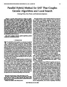
Fig. 2. Density function for a number of angles: (red dash(green dashed line) and (blue solid line). dotted line), and The black vertical lines denote the logarithmic singularities at for the case .
and the complete elliptic integral of the first kind. The Appendix also gives a convenient and easy way to numerically evaluate this special function. is proportional to the number of The density function sampling points of a translation operator that need to be evaluated in a particular -point. Expression (3) can be seen as the continuous approximation of the histogram that would represent this information for a finite [19]. is plotted for a number of different angles In Fig. 2, . In the Appendix it is proven that, for all generic angles , and ), has two logarithmic ( singularities at and . For or , the translation operator direction is parallel to is the uniform distribution. the -axis and, consequently, For , the translation direction is perpendicular to the -axis, resulting a single logarithmic singularity of at .
In short one can summarize the workflow of the sequential IM as presented in [4] as follows. in equidistant points in the interval • Evaluate using (1). We further refer to these points as interpolation points. • Compute the translation operator in the required sampling points by local interpolation using the points from the previous step. The number of source interpolation points needed to compute a single sampling point of the translation operator using local , i.e., independent of [20]. Consequently, interpolation is . the time complexity for both steps is The first step of the IM can be parallelized in a straightforgroups, ward way. First, the processes are subdivided in processes. As we are using each consisting of parallel processes, this corresponds to groups, where each processes. The interpolation points group contains are uniformly partitioned among these in the interval groups such that each group is responsible for the cominterpolation points. Explicitly, , the left putation of boundary point of process group , is determined by (with ). For this step no communication is required between groups. The computations within a group can be further parallelized: each process evaluates and terms in (1) for each interposums only a subset of the lation point in the group. This partitioning scheme is depicted time and there are no in Fig. 3. The computations take overlapping computations between processes. It is important to remark that we assume that spherical Hankel functions and Letime, gendre polynomials can be effectively evaluated in regardless of the order , ranging from 0 to . For the spherical Hankel functions, the Amos library [21] can be used. For the Legendre polynomials, such a method was recently developed in [16]. To complete the first step, the partial results need to be summed over all processes within a group. This summation, which of course does require communication, is performed in such a way that the resulting sum for each interpolation point in the group is present in each process of the group. In parallel computing, this operation is referred to as an all-reduce time [22]. As operation, which can be performed in this is the dominating complexity, the first step of the PIM also time. At the end of the first step, each process requires contains the evaluated interpolation points that correspond to the group to which the process belongs. In other words, the calculated interpolation points are redundantly stored in each process of a group, however, the computations themselves are not duplicated between processes. Conceptually, the parallelization of the second step of the IM is trivial: each process computes the translation operator in the sampling points of its local blockwise partition required
2682
IEEE TRANSACTIONS ON ANTENNAS AND PROPAGATION, VOL. 62, NO. 5, MAY 2014
Fig. 3. Parallelization concept of the first step of the PIM algorithm: the interpolation points are distributed among groups of parallel processes (horizontal solid lines). The computation of each of these interpolation terms between the propoints is further parallelized by splitting the cesses within each group (vertical solid lines). Each process hence computes terms for interpolation points. These terms are summed over all processes in a group using an all-reduce operation.
by local interpolation using the points generated in step 1. As sampling points of a process requires ineach of the terpolation points, it follows that each process needs only interpolation points in total to perform this second step. No dependencies between computations exist and hence, no communication between processes is required. However, prior to this second step, a mismatch exists between the subset of interpolation points that is required by a certain process to perform its computations in step 2 and the interpolation points that are actually present in local memory of that process at the end of step 1. Therefore, a communication phase has to take place in between both steps in which the interpolation points are redistributed among the processes. As each process interpolation points in step 2, it follows that requires only the total volume of data received by any process during this . In the next section, reshuffling phase is also bounded by we show that the total volume of data to be sent by a process is . bounded by B. Volume of Data to be Sent During the Reshuffling Phase In step 1, the interpolation points in the interval are uniformly partitioned among the groups. Fig. 4 illustrates the uniform partitioning for several density functions . corresponding to different values of is proportional to the Recall that the density function number of sampling points of the translation operator that depend on the value of . As the density function is non-uniform in general, certain interpolation points are required by more sampling points (and hence more processes) than others, giving rise to non-uniform communication patterns during the reshuffling of interpolation points in between steps 1 and 2. To determine the communication complexity, we consider the worst, i.e., at case scenario which occurs at the singularities of and . Consider the process group that contains the interpolation points around such a singularity, namely the interval , with .
Fig. 4. Uniform partitioning of the interpolation points as a function of among process groups (16 in this example). The vertical lines denote the is shown for partition boundaries. Additionally, the density function (blue solid line), (green dashed line) and (red dot-dashed line).
The total number of translation operator sampling points that correspond to these -values is proportional to (5a) (5b) (5c) (5d) around where we used an approximation of (derived in the Appendix) in (5b), in (5c) and the fact in (5d). From (5d) one sees that, in the that sampling points that worst-case scenario, there are depend on the -interval of a single process group.As there are processes in that group that can deliver this data, data in between steps no process has to send more than 1 and 2 when these communications are equally divided among processes. the We conclude that the volume of data to be sent by any process . in between the two steps is bounded by C. Summary of the Parallel Algorithm The steps of the parallel algorithm to calculate a translation operator can be summarized as follows: • Step 1a: Assign interpolation points to each group of processes. Each process within each group computes only a subset of the terms of (1) for each of the interpolation . points in the group. Cost: • Step 1b: Perform the parallel summation (all-reduce opera. tion) over all processes within each group. Cost: • Reshuffling phase: Interpolation points are redistributed receive volume for each among processes. Cost: process, send volume for the processes near the . singularities of • Step 2: Compute the translation operator in its sampling . points using local interpolation. Cost:
MICHIELS et al.: WELL-SCALING PARALLEL ALGORITHM FOR THE COMPUTATION OF THE TRANSLATION OPERATORIN THE MLFMA
2683
Assuming that all computations and communications by the different processes can be performed concurrently, the global . complexity of the parallel algorithm is IV. NUMERICAL RESULTS In this section, the implementation and the scaling behavior of the proposed PIM is numerically validated. The numerical data has been obtained using a cluster consisting of 256 machines each containing two 8-core Intel Xeon E5–2670 processors (4096 CPU-cores in total). The machines were connected using an FDR Infiniband network. To produce the results for , each CPU-core has been oversubscribed by 4 processes. The calculations were performed in double-precision. A. Validation of the Implementation To validate the implementation of the parallel computation of the proposed PIM algorithm, we consider the plane wave decomposition of the Green’s function [2], [3]
Fig. 5. Maximum relative error of the addition theorem as a function of partitions .
(6) with
. The factor is the aggregation, with . We chose and . For the target precision in (2) we consider three values: , and . The translation operators are calculated for the same values of and as in Table I, extended with and . The total number of interpolation points in the interval is set to . The - and -dimensions are sampled and points respectively, and as a result the in translation operators contain a total number of sampling points. These sampling rates are realistic, as they correspond to the actual sampling rates that are used in our MLFMA simulations. The local interpolation method is based on the product of the Dirichlet kernel and a Gaussian function [3][p. 65]. The number of neighboring interpolation points is chosen sufficiently high, so that the local interpolation is accurate up to machine precision. This way, the error of the addition theorem is only determined by the value of . As discussed, the communication of the interpolation points and hence on the in the PIM algorithm strongly depends on translation direction . Therefore, we consider the following 26 translation directions: (7) , 0 and where , and take all combinations of the values . 1, except the case Fig. 5 shows the maximum relative error of the addition theorem as a function of the number of partitions . As one can see, the obtained precision of the worst-case translation direction corresponds well to the target precision. The translation operators produced by the PIM are identical to the ones obtained through the sequential IM. B. Runtime Benchmark Table II shows the average runtime of the translation operators that were computed in the previous section, up to
TABLE II RUNTIME TO COMPUTE A TRANSLATION OPERATOR FOR AN INCREASING ( ) FOR THE PROPOSED PIM ALGORITHM
. The values for and are the same as in Table I and, therefore, the runtimes can be compared. First, by comparing the values in Tables I and II, one observes that for high values of the proposed PIM algorithm is roughly 10 times faster than the baseline PDM. This is a manifestation of the fact that the PIM has a lower time complexity, namely , with respect to the complexity of the PDM. When considering problems with billions of unknowns, such as the one presented in [11], the runtime for the computation of all translation operators during the setup stage is reduced from approximately one hour (PDM) to only a few minutes (PIM). With an overall runtime (setup time + solution time) for this simulation of about 45 hr, it is clear that even though this reduction is important, the relative reduction in overall runtime is modest. However, because the proposed PIM reduces the computational complexity, we expect that this gain in performance will become relatively more important when even larger simulations are considered. Second, one can see that the runtime of the PIM increases for a higher number of parallel processes faster than . This is caused by a limitation in the interconnection network of the cluster that was used. Specifically, the network supports only a limited number of concurrent communications between processes, which can cause a serialization of the communication and result in a slowdown of a factor two during the communication stage. Hence, we obtain runtimes for the PIM that are higher than expected, when using 1024 and 4096 processes.
2684
IEEE TRANSACTIONS ON ANTENNAS AND PROPAGATION, VOL. 62, NO. 5, MAY 2014
Fig. 6. Normalized number of interpolation points per process group for in). creasing and (with
C. Validation of the Theoretical Complexities In this section we want to numerically validate the theoretically derived complexities of the PIM. The same translation directions of (7) are used and the values corresponding to the worst-case are selected, just as in Section IV-A, in which the implementation has been validated. is set to , This time, the number of multipoles , instead of using (2). This way, a purely linear with is obrelationship between the number of multipoles and ). tained, which corresponds to the high-frequency limit ( is purely arbitrary, the resulting number of interpolation As . By enforcing a points can be normalized with respect to and , the asymppurely linear dependency between totic behavior of the proposed PIM becomes apparent for lower values of . Note that exactly the same conclusions will be obtained if (2) is used to calculate . Fig. 6 shows the number of interpolation points per process group as a function of , normalized by . As expected for uniform partitioning, this value is the same for each group and constant for an increasing number of and . The maximum normalized number of interpolation points to be received by a process, in order to compute its local translation operator sampling points, is shown in Fig. 7. For increasing and it is bounded by , as a result of the blockwise partitioning of the translation sampling points. Fig. 8 displays the total number of interpolation points a and , i.e., the process group has to send, divided by number of processes a group contains. In case of uniform or, equivalently, partitioning this is proportional to , which corresponds exactly to the behavior predicted by the theory. The results of this section show that the numerically obtained data corresponds very well to the theoretically predicted scaling behavior of the PIM. V. CONCLUSION In this paper the distributed-memory parallelization of the calculation of the translation operator in the MLFMA by means of the interpolation method was studied. To calculate a translamultipoles using processes, tion operator with
Fig. 7. Maximum normalized number of interpolation points required by a process in order to perform the local interpolation of its local translation sampling points.
Fig. 8. Total number of interpolation points a process group has to send, norand . malized by
our proposed algorithm requires only time, which is complexity of the basea clear improvement over the line parallel algorithm. The average time to compute a translation operator using the parallel interpolation method is measured using 4096 CPU-cores and compared to a parallel implementation of the baseline method. As a result, a large speedup factor for realistic electromagnetic problems is achieved, which reduces the time of the setup stage significantly. Furthermore, the theoretical results for the parallel interpolation method were processes and its scaling numerically verified using up to behavior corresponded very well to the theoretical analysis. APPENDIX In this appendix, an expression for the density function of the translation sampling points as a function of is derived. Density Function: From Fig. 1 one sees that there is an accumulation of sampling points at the poles of the sphere, due to the uniform sampling in and . As a result, one obtains a non-uniform distribution of the sampling points as a function of that depends on , the direction of the translation.
MICHIELS et al.: WELL-SCALING PARALLEL ALGORITHM FOR THE COMPUTATION OF THE TRANSLATION OPERATORIN THE MLFMA
Consider the asymptotic case with and choose the -coordinate system so that , with . As the Jacobian of a spherical coordinate system on the unit sphere and as the sampling points are uniformly is equal to , the density of the sampling points is sampled in
2685
Finally, after numerous yet straightforward algebraic operations, one obtains
(16a)
(8a) (16b) (8b) Now consider the coordinate system of the translation direction, . Using a rotation over the where the -axis is parallel to about the -axis, can be expressed in this coangle ordinate system as
and the complete elliptic integral with of the first kind [23]. Using (10) and the definitions of and , one finds the expression of (3). and one sees that For the special cases
(9)
(17a) (17b)
The density function of the translation sampling points as a is equal to function of
(17c)
(10) is the radius of a circle of latitude in the coordinate as system of . In the special case when or , degenerates to (11a) (11b) (11c) Elliptic Integral: To find an expression for the density one has to calculate the integral function
as (11).
. This result corresponds to the result of
Singularities: The complete elliptic integral of the first [23] kind has a logarithmic singularity in (18) has a From (3), one can derive that the density function and , except logarithmic singularity in and . for the degenerate cases is not very close to 0 or . After a second Assume that order Taylor expansion of the argument of the elliptic integral and substituting in the non-singular around one obtains part of (19a) (19b)
(12) with As
and ranges from , one can write
to
with
. in the interval
(20a) (20b) (13)
The key to simplify the integrand is the substitution (14) The variable
is a positive real number, as
. The approximation of (19) is valid as long as one can derive a similar For the singularity in expression. Numerical Evaluation: The appearance of an elliptic intedoes not gral in the expression of the density function pose a problem because it can be easily and quickly computed using (21)
(15) is smaller than 1 when ranges from to 0.
. For
,
with the arithmetic-geometric mean [23]. For completeness, we also mention that one should be very close to its singularity at careful when evaluating
2686
IEEE TRANSACTIONS ON ANTENNAS AND PROPAGATION, VOL. 62, NO. 5, MAY 2014
as the expression of (16b) would lead to numerical inaccuracies. To understand this, we consider
(22a) (22b) (22c)
with (23a) (23b) When is close to pansion
one can use a second order Taylor ex-
(24) is in the region of Suppose a machine precision . When , the evaluation of already reaches machine precicomes closer to , the second factor of (23b) will sion. If be rounded to 0 or . This is clearly undesirable for the compuand tation of the arithmetic-geometric mean will lead to numerical inaccuracies in the calculation of the el. liptic integral Therefore, the numerator of (22c) has to be rewritten as (25) This expression does not suffer from a numerical breakdown and it allows to obtain accurate results when computing numerically. ACKNOWLEDGMENT The computational resources (Stevin Supercomputer Infrastructure) and services used in this work were provided by Ghent University, the Hercules Foundation and the Flemish Government – department EWI.
[6] L. Gürel and Ö. Ergül, “Hierarchical parallelization of the multilevel fast multipole algorithm (MLFMA),” Proc. IEEE, vol. 101, no. 2, pp. 332–341, Feb. 2013. [7] Ö. Ergül and L. Gürel, “Accurate solutions of extremely large integralequation problems in computational electromagnetics,” Proc. IEEE, vol. 101, no. 2, pp. 342–349, Feb. 2013. [8] J. M. Taboada, M. G. Araujo, F. Obelleiro, J. L. Rodriguez, and L. Landesa, “MLFMA-FFT parallel algorithm for the solution of extremely large problems in electromagnetics,” Proc. IEEE, vol. 101, no. 2, pp. 350–363, Feb. 2013. [9] X. M. Pan, W. C. Pi, M. L. Yang, Z. Peng, and X. Q. Sheng, “Solving problems with over one billion unknowns by the MLFMA,” IEEE Trans. Antennas Propag., vol. 60, no. 5, pp. 2571–2574, May 2012. [10] B. Michiels, J. Fostier, I. Bogaert, and D. De Zutter, “Weak scalability analysis of the distributed-memory parallel MLFMA,” IEEE Trans. Antennas Propag., vol. 61, no. 11, pp. 5567–5574, Nov. 2013. [11] B. Michiels, J. Fostier, I. Bogaert, and D. De Zutter, “Full-wave simulation of electromagnetic scattering problem with more than three billion unknowns,” IEEE Trans. Antennas Propag., 2014, submitted for publication. [12] Ö. Ergül and L. Gürel, “Hierarchical parallelisation strategy for multilevel fast multipole algorithm in computational electromagnetics,” Electron. Lett., vol. 44, no. 1, pp. 3–4, Jan. 2008. [13] Ö. Ergül and L. Gürel, “A hierarchical partitioning strategy for an efficient parallelization of the multilevel fast multipole algorithm,” IEEE Trans. Antennas Propag., vol. 57, no. 6, pp. 1740–1750, Jun. 2009. [14] J. Fostier and F. Olyslager, “Provably scalable parallel multilevel fast multipole algorithm,” Electron. Lett., vol. 44, no. 19, pp. 1111–1112, Sep. 2008. [15] B. Michiels, J. Fostier, I. Bogaert, P. Demeester, and D. De Zutter, “Towards a scalable parallel MLFMA in three dimensions,” in Proc. Computat. Electromagnet. Int. Workshop (CEM ’11), Izmir, Turkey, Aug. 2011, pp. 132–135. [16] I. Bogaert, B. Michiels, and J. Fostier, “ computation of Legendre polynomials and Gauss-Legendre nodes and weights for parallel computing,” SIAM J. Scientif. Comput., vol. 34, no. 3, pp. C83–C101, 2012. [17] J. Sarvas, “Performing interpolation and anterpolation entirely by fast Fourier transform in the 3-D multilevel fast multipole algorithm,” SIAM J. Numerical Anal., vol. 41, no. 6, pp. 2180–2196, 2003. [18] L. Gürel and Ö. Ergül, “Fast and accurate solutions of extremely large integral-equation problems discretised with tens of millions of unknowns,” Electron. Lett., vol. 43, no. 9, pp. 499–500, Apr. 2007. [19] B. Michiels, I. Bogaert, J. Fostier, and D. De Zutter, “A weak scalability study of the parallel computation of the translation operator in the MLFMA,” in Proc. Int. Conf. Electromagnet. in Advanced Applicat. (ICEAA 2013), Turin, Italy, Sep. 2013, pp. 369–399. [20] O. M. Bucci, C. Gennareli, and C. Savarese, “Optimal interpolation of radiated fields over a sphere,” IEEE Trans. Antennas Propag., vol. 39, no. 11, pp. 1633–1643, Nov. 1991. [21] D. E. Amos, “A portable package for Bessel functions of a complex argument and nonnegative order,” ACM Trans. Math. Softw. (TOMS), vol. 12, no. 3, pp. 265–273, Sep. 1986. [22] R. Thakur and R. Rabenseifner, “Optimization of collective communication operations in MPICH,” Int. J. High Performance Comput. Applicat., vol. 19, pp. 49–66, 2005. [23] F. Olver, D. Lozier, R. Boisvert, and C. Clark, NIST Handbook Of Mathematical Functions. New York, NY, USA: Cambridge Univ. Press, 2010.
REFERENCES [1] L. Greengard and V. Rokhlin, “A fast algorithm for particle simulations,” J. Computat. Phys., vol. 73, no. 2, pp. 325–348, Dec. 1987. [2] R. Coifman, V. Rokhlin, and S. Wandzura, “The fast multipole method for the wave equation: A pedestrian prescription,” IEEE Antennas Propag. Mag., vol. 35, no. 3, pp. 7–12, Jun. 1993. [3] W. C. Chew, J. Jin, E. Michielssen, and J. Song, Fast and Efficient Algorithms in Computational Electromagnetics. London, U.K.: Artech House, 2001. [4] J. Song and W. C. Chew, “Interpolation of translation matrix in MLFMA,” Microw. Opt. Technol. Lett., vol. 30, no. 2, pp. 109–114, Jul. 2001. [5] Ö. Ergül and L. Gürel, “Optimal interpolation of translation operator in multilevel fast multipole algorithm,” IEEE Trans. Antennas Propag., vol. 54, no. 12, pp. 3822–3826, Dec. 2006.
Bart Michiels was born on October 30, 1986. He received the M.S. degree in engineering physics from Ghent University, Ghent, Belgium, in 2009. His master’s thesis dealt with the simulation of large, broadband two-dimensional electromagnetic problems, using the Multilevel Fast Multipole Method (MLFMA). In 2013, he received the Ph.D. degree in engineering physics from the Department of Information Technology (INTEC) in Ghent. The main topic of his Ph.D. thesis was the parallelization of the MLFMA and its parallel scalability, in order to solve large-scale full-wave electromagnetic problems.
MICHIELS et al.: WELL-SCALING PARALLEL ALGORITHM FOR THE COMPUTATION OF THE TRANSLATION OPERATORIN THE MLFMA
Ignace Bogaert (S’07–M’12) was born in Ghent, Belgium, in 1981. He received the M.S. degree in engineering physics from Ghent University, Ghent, in 2004. After graduating, he joined the Electromagnetics Group of the Department of Information Technology (INTEC) at Ghent University, where he received his Ph.D. degree in applied physics in 2008. His research is supported by a postdoctoral grant from the Research Foundation-Flanders (FWO-Vlaanderen). His research interests include optimization problems and the modeling of various physical systems, with the emphasis on robustness, efficiency and accuracy.
Jan Fostier (M’10) was born in 1982. He received the M.S. degree in physical engineering in 2005 and the Ph.D. degree in applied physics in 2009, both from Ghent University, Ghent, Belgium. In 2005, he joined the electromagnetics research group at the Department of Information Technology (INTEC) and in 2011 he was appointed Assistant Professor at the Internet Based Communication Networks and Services (IBCN) research group at the same department. His current research interests are numerical techniques, fast algorithms and distributed computing for bio-informatics and electromagnetics problems.
2687
Daniël De Zutter (M’92–SM’96–F’01) was born in 1953. He received the M.Sc. degree in electrical engineering from the University of Gent, Ghent, Belgium, in 1976. In 1981 he received the Ph.D. degree and in 1984 he completed a thesis leading to a degree equivalent to the French Aggrégation or the German Habilitation (both at the University of Gent). He is now a full Professor of Electromagnetics. His research focusses on all aspects of circuit and electromagnetic modelling of high-speed and high-frequency interconnections and packaging, on electromagnetic compatibility (EMC) and numerical solutions of Maxwell’s equations. As author or co-author he has contributed to more than 200 international journal papers (cited in the Web of Science) and 200 papers in conference proceedings. He was an Associate Editor for the IEEE TRANSACTIONS ON MICROWAVE THEORY AND TECHNIQUES. Between 2004 and 2008 he served as the Dean of the Faculty of Engineering of Ghent University and is now the head of the Department of Information Technology.