Active Learning for Automatic Classification of Software Behavior James F. Bowring
James M. Rehg
Mary Jean Harrold
College of Computing Georgia Institute of Technology Atlanta, Georgia 30332-0280
College of Computing Georgia Institute of Technology Atlanta, Georgia 30332-0280
College of Computing Georgia Institute of Technology Atlanta, Georgia 30332-0280
[email protected]
[email protected]
[email protected]
ABSTRACT
1.
A program’s behavior is ultimately the collection of all its executions. This collection is diverse, unpredictable, and generally unbounded. Thus it is especially suited to statistical analysis and machine learning techniques. The primary focus of this paper is on the automatic classification of program behavior using execution data. Prior work on classifiers for software engineering adopts a classical batchlearning approach. In contrast, we explore an active-learning paradigm for behavior classification. In active learning, the classifier is trained incrementally on a series of labeled data elements. Secondly, we explore the thesis that certain features of program behavior are stochastic processes that exhibit the Markov property, and that the resultant Markov models of individual program executions can be automatically clustered into effective predictors of program behavior. We present a technique that models program executions as Markov models, and a clustering method for Markov models that aggregates multiple program executions into effective behavior classifiers. We evaluate an application of active learning to the efficient refinement of our classifiers by conducting three empirical studies that explore a scenario illustrating automated test plan augmentation.
Software engineers seek to understand software behavior at all stages of development. For example, during requirements analysis they may use formal behavior models, usecase analysis, or rapid prototyping to specify software behavior [3, 16]. After implementation, engineers aim to assess the reliability of software’s behavior using testing and analysis. Each of these approaches evaluates behavior relative to a particular development phase, thereby limiting the range of behaviors considered. We believe that a program’s behavior is richer and more complex than the characterization provided by these perspectives. Software behavior is ultimately the collection of all its executions, embodying the diversity of all users, inputs, and execution environments for all copies of the program. This collection is unpredictable and generally unbounded, and thus requires a data-driven approach to analysis. Our approach to understanding behavior is to build behavior models from data using statistical machinelearning techniques. For any program, there exist numerous features for which we can collect aggregate statistical measures, such as branch profiles. If these features are accurate predictors of program behavior, then a broad range of statistical machine-learning techniques [17] could be used to aid analysis tasks such as automated-oracle testing, evaluation of test plans, detection of behavior profiles in deployed software, and reverse engineering. The focus of this paper is on the automatic classification of program behavior using execution data. In this context, a classifier is a map from execution statistics such as branch profiles to a label for program behavior such as “pass” or “fail”. Three issues must be addressed during classifier design: 1) a set of features, 2) a classifier architecture, and 3) a learning technique for training the classifier using labeled data [17]. For example, in recent work by Podgurski and colleagues [20], a classifier based on logistic regression uses composite features from execution profiles to identify failures that may share a common fault. The application of machine learning techniques such as classification to software engineering problems is relatively new (some representative examples are [1, 4, 7, 14, 11, 15, 20]). All of this prior work adopts a classical batchlearning approach, in which a fixed quantity of manuallylabeled training data is collected at the start of the learning process. In contrast, the focus of this paper is on an activelearning paradigm [5] for behavior classification. In active
Categories and Subject Descriptors D.2.4 [Software Engineering]: Software/Program Verification; G.3 [Mathematics of Computing]: Probability and Statistics; I.2.6 [Artificial Intelligence]: Learning
General Terms Measurement, Reliability, Experimentation, Verification
Keywords Software testing, software behavior, machine learning, Markov models
Permission to make digital or hard copies of all or part of this work for personal or classroom use is granted without fee provided that copies are not made or distributed for profit or commercial advantage and that copies bear this notice and the full citation on the first page. To copy otherwise, to republish, to post on servers or to redistribute to lists, requires prior specific permission and/or a fee. ISSTA’04, July 11–14, 2004, Boston, Massachusetts, USA. Copyright 2004 ACM 1-58113-820-2/04/0007 ...$5.00.
INTRODUCTION
learning, the classifier is trained incrementally on a series of labeled data elements. During each iteration of learning, the current classifier is applied to the pool of unlabeled data to predict those elements that would most significantly extend the range of behaviors that can be classified. These selected elements are then labeled and added to the training set for the next round of learning. The potential advantage of active learning in the softwareengineering context is the ability to make more effective use of the limited resources that are available for analyzing and labeling program execution data. If an evolving classifier can make useful predictions about which data items are likely to correspond to new behaviors, then those items can be selected preferentially. As a result, the scope of the model can be extended beyond what a batch method would yield, for the same amount of labeling effort. We have found empirically that active learning can yield classifiers of comparable quality to those produced by batch learning with a significant savings in data-labeling effort. In addition, we have found that the data items selected during active learning can be used to more efficiently extend the scope of test plans. These are important findings because human analysis of program outputs is inherently expensive, and many machine learning techniques depend for their success on copious amounts of labeled data. A second contribution of this paper is an investigation of whether features derived from Markov models of program execution can adequately characterize a specific set of behaviors, such as those induced by a test plan. Specifically, we explore the thesis that the sequence of method calls and branches in an executing program is a stochastic process that exhibits the Markov property. The Markov property implies that predictions about future program states depend only upon the current state. Method caller/callee transitions and branches together form the basic set of arcs in interprocedural control-flow graphs 1 (ICFGs). These features are part of the larger feature set used in References [7, 20]. Furthermore, branch profiles have been shown to be good detectors of the presence of faults by other researchers (e.g., [13, 23]). We specify Markov models of program behavior based on these features. Previous works (e.g., [7, 20]) have demonstrated the power of clustering techniques in developing aggregate descriptions of program executions. We present an automated clustering method for Markov models that aggregates multiple program executions. Each resulting cluster is itself a Markov model that is a statistical description of the collection of executions it represents. With this approach, we train classifiers to recognize specific behaviors emitted by an execution without knowledge of inputs or outcomes. There are two main benefits of our work. First, we show that modeling certain event transitions as Markov processes produces effective predictors of behavior that can be automatically clustered into behavior classifiers. Secondly, we show that these classifiers can be efficiently evolved with the application of active-learning techniques.
1 An interprocedural control-flow graph is a directed graph consisting of a control-flow graph for each method plus edges connecting methods to call sites and returns from calls. A control-flow graph is a directed graph in which nodes represent statements or basic blocks and edges represent the flow of control.
The contributions of this paper are: • A technique that automatically clusters Markov models of program executions to build classifiers. • An application of our technique that efficiently refines our classifiers using active learning (bootstrapping) and a demonstration of the application to an example of automated test plan augmentation. • A set of empirical studies that demonstrate that the classifiers built by our technique from Markov models are both good predictors of program behavior and good detectors of unknown behaviors.
2.
RELATED WORK
The previous work that is closest in spirit and method to our work is that of Podgurski and colleagues [7, 20]. Their work uses clustering techniques to build statistical models from program executions and applies them to the tasks of fault detection and failure categorization. The two primary differences between our technique and this previous work are the central role of Markov models in our approach and our use of active learning techniques to improve the efficiency of behavior modeling. An additional difference is that we explore the utility of using one or two features instead of a large set of features. Dickinson, Leon, and Podgurski demonstrate the advantage of automated clustering of execution profiles over random selection for finding failures [7]. They use many feature profiles as the basis for cluster formation. We concentrate on two features that summarize event transitions—method caller/callee profiles and branch profiles. We show the utility of Markov models based on these profiles as predictors of program behavior. In Podgurski et al. [20], clustering is combined with feature selection, and multidimensional scaling is used to visualize the resulting grouping of executions. In both of these works, the clusters are formed once using batch learning and then used for subsequent analysis. In contrast, we explore an active learning technique that interleaves clustering with evaluation for greater efficiency. Another group of related papers share our approach of using Markov models to describe the stochastic dynamic behavior of program executions. Whittaker and Poore use Markov chains to model software usage from specifications prior to implementation [24]. In contrast, we use Markov models to describe the statistical distribution of transitions measured from executing programs. Cook and Wolf confirm the power of Markov models as encoders of individual executions in their study of automated process discovery from execution traces [6]. They concentrate on transforming Markov models into finite state machines as models of process. In comparison, our technique uses Markov models to directly classify program behaviors. Jha, Tan, and Maxion use Markov models of event traces as the basis for intrusion detection [15]. They address the problem of scoring events that have not been encountered during training, whereas we focus on the role of clustering techniques in developing accurate classifiers. The final category of related work uses a wide range of alternative statistical learning methods to analyze program executions. Although the models and methods in these works differ substantially from ours in detail, we share a common goal of developing useful characterizations of aggregate program behaviors. Harder, Mellen, and Ernst automatically classify software behavior using an operational
Stage 1. Prepare Training Instances
Stage 2. Train Classifier
Program P
Instrument P to profile event transitions
^ P
Execute & Label Behaviors
Training Instances = Event Transition Profiles w/ Behavior Labels
Group by Behavior Labels
Test Plan w/ Behavior Oracle
Behavior Groups b1,…,bn
Train one Classifier per Group
Classifiers Cb1,…,Cbn
Assemble Classifier C for P
Classifier C
Figure 1: Building Classifier: Stage 1 - Prepare Training Instances; Stage 2 - Train Classifier. differencing technique [12]. Their method extracts formal operational abstractions from statistical summaries of program executions and uses them to automate the augmentation of test suites. In comparison, our modeling of program behavior is based exclusively on the Markov statistics of events. Brun and Ernst use dynamic invariant detection to extract program properties relevant to revealing faults and then apply batch learning techniques to rank and select these properties [4]. However, the properties they select are themselves formed from a large number of disparate features and the authors’ focus is only on fault-localization and not on program behavior in general. In contrast, we seek to isolate the features critical to describing various behaviors. Additionally, we apply active learning to the construction of the classifiers in contrast to the batch learning used by the authors. Gross and colleagues propose the Software Dependability Framework, which monitors running programs, collects statistics, and, using multivariate state estimation, automatically builds models for use in predicting failures during execution [11]. This framework does not discriminate among features, where we do and consequently we use Markov statistics of events instead of multivariate estimates to model program behavior. Their models are built once use batch learning whereas we demonstrate the advantages of active learning. Munson and Elbaum posit that actual executions are the final source of reliability measures [18]. They model program executions as transitions between program modules, with an additional terminal state to represent failure. They focus on reliability estimation by modeling the transition probabilities into the failure state. We focus on behavior classification for programs that may not have a well-defined failure state. Ammons, Bodik, and Larus describe specification mining, a technique for extracting formal specifications from interaction traces by learning probabilistic finite suffix automata models [1]. Their technique recognizes the stochastic nature of executions, but it focuses on extracting invariants of behavior rather than mappings from execution event statistics to behavior classes.
3.
MODELING SOFTWARE BEHAVIOR
Our goal is to build simple models of program behavior that will reliably summarize and predict behavior. To do
this, we focus on the subset of features that profile event transitions in program executions. An event transition is a transition from one program entity to another; types of 1st-order event transitions include branches (source statement to sink statement), method calls (caller to callee), and definition-use pairs (definition to use); one type of 2nd-order event transition is branch-to-branch. An event-transition profile is the frequency with which an event transition occurred during an execution. We show that these event-transition features describe stochastic processes that exhibit the Markov property by building Markov models from them that effectively predict program behavior. The Markov property provides that the probability distribution of future states of a process depends only upon the current state. Thus, a Markov model captures the time-independent probability of being in state s1 at time t+1 given that the state at time t was s0 . The relative frequency of an event transition during a program execution provides a measure of its probability. For instance, a branch is an event transition in the control-flow graph2 (CFG) of a program between a source node and a sink node. The source and sink nodes are states in the Markov model. For a source node that is a predicate there are two branches, true and false, each representing a transition to a different sink node. The transition probabilities in the Markov model between this source node and the two sink nodes are the relative execution frequencies, or profiles, of the branches. In general, the state variables could represent other events such as variable definitions and variable uses. The state variables could also represent more complex event sets such as paths of length two or more between events. Paths of length two are referred to as 2nd-order event transitions. The profiling mechanism would collect frequency data for transitions between these events for use in the Markov models. An area of future research is to examine the trade-offs between the costs of collecting higher-order event-transition profiles and the benefits provided by their predictive abilities. Our technique (Figure 1) builds a classifier for software behavior in two stages. Initially, we model individual program executions as Markov models built from the profiles of event transitions such as branches. Each of these mod2
A control-flow graph is a directed graph in which nodes represent statements or basic blocks and edges represent the flow of control.
els thus represents one instance of the program’s behavior. The technique then uses an automatic clustering algorithm to build clusters of these Markov models, which then together form a classifier tuned to predict specific behavioral characteristics of the considered program. Figure 1 shows a data-flow diagram of our technique. In the data-flow diagram, the boxes represent external entities, (i.e., inputs and outputs), and the circles represent processes. The arrows depict the flow of data and the parallel horizontal lines in the center are a database. Reading the diagram from left to right, the technique takes as inputs a subject program P , its test plan, and its behavior oracle, and outputs a Classifier C. P ’s test plan contains test cases that detail inputs and expected outcomes. The behavior oracle evaluates an execution ek of P induced by test case tk and outputs a behavior label bk , such as, but not restricted to, “pass” or “fail.” In Stage 1, Prepare Training Instances, the technique instruments P to get Pˆ so that as Pˆ executes, it records eventtransition profiles. For each execution ek of Pˆ with test case tk , the behavior oracle uses the outcome specified in tk to evaluate and label ek . This produces a training instance— consisting of ek ’s event-transition profiles and its behavior label—that is stored in a database. In Stage 2, Train Classifier, the technique first groups the training instances by the distinct behavior labels b1 , . . . , bn generated by the behavior oracle. For example, if the behavior labels are “pass” and “fail,” the result is two behavior groups. Then, the technique converts each training instance in each behavior group to a Markov model. The technique initially uses a batch-learning paradigm to train one classifier Cbk per behavior group bk . Finally, the technique assembles the behavior group classifiers, Cb1 , . . . , Cbn to assemble the classifier C for P . Before exploring the algorithm TrainClassifier, shown in Figure 4, we discuss Markov model building.
3.1
Building Markov Models
Central to our technique is the use of Markov models to encode the event-transition profiles produced by Pˆ . The transformation is a straightforward mathematical process, but it is important to understand the mapping from program events to the concept of state that we use in building the Markov models. To illustrate, consider the CFG in Figure 2. The branch profiles for an arbitrary example execution e1 are shown in the labels for each branch. For example, branch B1’s profile denotes that it was exercised nine times. The Markov model built from this execution is also shown in Figure 2 as a matrix. It models the program states identified by the source and sink nodes of each branch. The transitions are read from row to column. A Markov model built from branch profiles is simply the adjacency matrix of the CFG with each entry equal to the row-normalized profile. For instance, node p1 is the source of two transitions, branches B1 and B2, which occur a total of ten times. As an example implementation of the transformation, we present algorithm BuildModel, shown in Figure 3. BuildModel constructs a matrix representation of a Markov model from event-transition profiles. Note that as the number of states specified in the Markov model increases, efficiency will dictate the use of a more sparse representation than that of conventional matrices.
Entry
Branch B2 Profile = 1
Entry Arc Profile = 1
F
p1 Branch B1 Profile = 9
Exit
T
p2
Branch B3 Profile = 3
T
Branch B4 Profile = 6
F
s2
s1 s3
Markov Model of Branch Profiles p2
s1
s2
Entry
Entry p1 0
1/1
0
0
0
Exit 0
p1
0
0
9 / 10
0
0
1 / 10
p2
0
0
0
3/9
6/9
0
s1
0
1/1
0
0
0
0
s2 Exit
0
1/1
0
0
0
0
0
0
0
0
0
1/1
Figure 2: Representing branch profiles as a Markov model. BuildModel has three inputs: S, D, b. S is a set of states or events used to specify the event transitions. D contains the event transitions and their profiles stored as ordered triples, each describing a transition from a state sf rom to a state sto with the corresponding profile: (sf rom , sto , prof ile). b is the behavior label for the model. The output (M, D, b) is a triple of the model, the profile data, and the behavior label. In line 1, the matrix M for the model is initialized using the cardinality of S. In lines 2-3, each transition in D that involves states in S is recorded in M . In lines 4-8 each row in matrix M is normalized by dividing each element in the row by the sum of the elements in the row, unless the sum is zero. For the execution e1 shown in Figure 2, the inputs to BuildModel for 1st-order event transitions are: • S = {Entry, p1, p2, s1, s2, exit} • D = ((Entry, p1, 1), (p1, Exit, 1), . . . , (p2, s2, 6)) • b = “pass”
In this case, the output component M is the Markov model shown in Figure 2.
3.2
Training the Classifier
Our approach is to train a behavior classifier using as training instances the Markov models that we have constructed from the execution profiles. The training process we use is an adaptation of an established technique known
Algorithm BuildModel(S, D, b) Input: S = {s0 , s1 , . . . , sn }, a set of states, including a final or exit state, D = ((sf rom , sto , prof ile), . . . ), a list of ordered triples for each transition and its profile b = a string representing a behavior label Output:(M, D, b), a Markov model, D and b (1) (2) (3) (4) (5) (6) (7) (8) (9)
M ← new f loat Array[|S|, |S|], initialized to 0 foreach {sf rom , sto , prof ile} ∈ D, where s ∈ S M [sf rom , sto ] ← M [sf rom , sto ] + prof ile for i ← 0 to (|S| − 1) P|S|−1 rowSum ← j=0 M [i, j] if rowSum > 0 for j ← 0 to (|S| − 1) M [i, j] ← M [i, j]/rowSum return (M, D, b)
Figure 3: Algorithm to build model. as agglomerative hierarchical clustering [9]. With this technique, initially each training instance is considered to be a cluster of size one. The technique proceeds iteratively by finding the two clusters that are nearest to each other according to some similarity function. These two clusters are then merged into one, and the technique repeats. The stopping condition is either a desired number of clusters or some valuation of the quality of the remaining clusters. The specification of the similarity function is typically done heuristically according to the application domain. In our case, we need to specify how two Markov models can be compared. In the empirical studies presented in this paper, we choose a very simple comparison, which is the Hamming distance3 between the models. To compute the Hamming distance, each of the two Markov models is first mapped to a binary representation where a 1 is entered for all values above a certain threshold, and a 0 is entered otherwise. The threshold value is determined experimentally. We label the comparison function SIM and supply it as an input to our algorithm TrainClassifier shown in Figure 4 and discussed below. The binary transformation of the models is done only temporarily by SIM in order to compute the Hamming distance. Each merged cluster is also a Markov model. For example, in the first iteration, the merged model is built by combining the execution profiles that form the basis for the two models being merged. The profiles are combined by first forming their union, and then summing the values of redundant entries. Thus, if two executions were identical in their profiles, the result of combining the two profiles would be one profile with each entry containing a value twice that of the corresponding entry in the single execution. Referring to Figure 2, the merged profile for two copies of this execution would be: • D = ((Entry, p1, 2), (p1, Exit, 2), . . . , (p2, s2, 12))
Then from this merged profile, BuildModel generates a Markov model that represents the new cluster. For the stopping criterion, we have developed a simple heuristic that evaluates the stability of the standard deviation of the set of similarity measures that obtains at any given iteration. When the standard deviation begins to 3 The Hamming distance between two binary numbers is the count of bit positions in which they differ.
Algorithm TrainClassifier(S, T, SIM ) Input: S = {s0 , s1 , . . . , sn }, a set of states, including a final or exit state, T = ((testcasei , Di , bk ), . . . ), a list of ordered triples , where D = ((sf rom , sto , prof ile), . . . ), and b = a string representing a behavior label, SIM , a function to compute the similarity of two Markov models Output: C, a set of Markov models, initially ∅ (1) foreach (testcasei , Di , bk ) ∈ T , (2) 0 < i