ENHANCED SENSOR/ACTUATOR RESOLUTION AND ROBUSTNESS ANALYSIS FOR FDI USING THE EXTENDED GENERALIZED PARITY VECTOR TECHNIQUE Maira Omana and James H. Taylor
Abstract— This paper is an extension of the generalized parity vector (GPV) approach presented in Omana and Taylor [1]. Some aspects of sensor isolation are first clarified and a special case is defined to solve an important sensor/actuator fault detection and isolation (FDI) ambiguity issue. To overcome this problem, a new optimization constraint is incorporated in the transformation generation procedure used to improve separation in the generalized parity space. The validity of the different aspects analyzed through this research is demonstrated by testing this FDI scheme using a nonlinear jacketed continuously stirred tank reactor model. Robustness analysis is then performed over the controller envelope, showing the capability of the FDI technique to handle operating point and fault size variability.
I. INTRODUCTION The Generalized Parity Vector (GPV) technique is a modelbased approach based on the concept of analytical redundancy [2], [3], [4], [5], [6] and the use of linearized models. This paper deals with two long-standing questions in the use of the GPV technique for fault detection and isolation (FDI): sensor/actuator ambiguity and robustness [7]. The internal structure of some dynamic systems make it difficult to isolate certain pairs of sensor/actuator failures, and using linearized models in any context raises basic performance issues. If setpoint variation is large, then a significant deviation in the corresponding linearized model may occur, yielding a poor approximation of the nonlinear model at this new operating point. Most industrial processes require frequent operating point changes in order to satisfy production requirements [8], therefore modelling errors become a significant issue for this FDI method. This paper is outlined as follows: First, a brief overview of stable factorization and its application to implement the generalized parity vector technique is given in section II. Next, in section III, different cases for sensor and actuator FDI using directional residuals are defined [9], [10], [11]. Section IV presents an overview of the transformation matrix optimization method proposed in Omana and Taylor [1] and includes an extension to improve isolation for systems with sensor/actuator ambiguity. Finally, section V and VI present the FDI robustness studies with respect to operating point and fault size variability for a classical example, the jacketed continuously stirred tank reactor (JCSTR). Maira Omana is a MSc. candidate with the Department of Electrical & Computer Engineering, University of New Brunswick, PO Box 4400, Fredericton, NB CANADA E3B 5A3
[email protected] James H. Taylor is a Professor in the Department of Electrical & Computer Engineering, University of New Brunswick, PO Box 4400, Fredericton, NB CANADA E3B 5A3
[email protected]
II. R ESIDUAL G ENERATION USING THE G ENERALIZED PARITY V ECTOR T ECHNIQUE The residual generator is implemented using the generalized parity vector technique, which is developed in the stable factorization framework. The significance of using the stable coprime factorization approach is that the parity relations obtained involve stable, proper and rational transfer functions even for unstable plants. Therefore the realizability and stability of the residual generator is guaranteed. Given any nxm proper rational transfer function matrix P(s), it can be expressed in terms of its left coprime factors as follows [12]: ˜ −1 N ˜ (s) P (s) = D(s) (1) ˜ ˜ where N(s) and D(s) are called the left coprime factors and belong to the set of stable transfer function matrices. The GPV technique is based on the stable factorization of the system transfer function matrix in terms of its state-space representation. Let the system be described by the set of equations: x(t) ˙ = Ax(t) + Bu(t) + Gd(t)
(2)
y(t) = Cx(t) + Eu(t)
(3)
where x, u, d, and y represent the state variables, inputs, disturbances and outputs of the system, respectively. Assuming that the pairs (A, B) and (A, C) are stabilizable and detectable, it is possible to select a constant matrix F such that the matrix Ao , A − F C is stable. Using the definition of the coprime factorization of P(s) in [13], the left coprime factors are given by: ˜ = C(sI − Ao )−1 (B − F E) + E N (4) ˜ = I − C(sI − Ao )−1 F D
(5)
Based on the definition of the transfer function matrix P(s) given in equation (1) and taking the relationship among the desired control input, ud , and the actual output of the sensors, y, the following relations are obtained: ˜ −1 N ˜ (s) = y(s) (6) P (s) = D(s) ud (s) ˜ ˜ (s)ud (s) = 0 D(s)y(s) −N
(7)
Under ideal conditions, when the plant is linear, noise and fault free, equation (7) holds. However, when a fault happens, this relation is violated showing the inconsistency between the actuator inputs and sensor outputs with respect to the unfailed model.
Using this fact, the generalized parity vector, p(s), is defined as: ˜ ˜ (s)ud (s) ] p(s) = Tr [ D(s)y(s) −N (8)
achieved. However, for any system, the GPV always lies on a plane in the generalized parity space, defined by the vectors Edi and Bdi [7].
The GPV p(s) is a time varying function of small magnitude under normal operating conditions, due to the presence of noise and modeling errors arising from linearization and order reduction. However, it exhibits a significant magnitude change when a fault occurs. Each distinct failure produces a parity vector with different characteristics, allowing the use of the GPV for isolation purposes. A transformation matrix Tr (s) is introduced to make it possible to isolate faults more effectively [7].
The sensor fault isolation can be based on the angle Θi , between the GPV and the ith sensor reference plane, SP i , as illustrated in figure 2. If the ith sensor is faulty, this angle should be zero or less than Th .
N spi
GPV x3
Θi
SP i
III. FAULT D ETECTION AND I SOLATION USING DIRECTIONAL RESIDUALS
The basic idea of FDI using failure directions is that each failure will result in activity of the parity vector along certain axes or in certain subspaces. Depending on the dynamics of the system, some of these reference directions may be close or identical, making the isolation for some faults difficult or unachievable. To overcome the angle separation problem between the reference directions, the calculation of an optimal transformation matrix Tr is introduced in section IV. A. Actuator Faults Assuming an additive fault aj (t) in the j th actuator and using the definitions in section II, the GPV becomes: ˜ )j aj (s) , Tr Bnj aj (s) pa,j (s) = −(Tr N (9) s+σ Equation (9) shows that pa,j (s) is restricted to exhibit activity ˜ which along the direction defined by the j th column of N, we denote Bnj [7]. Actuator fault isolation is thus based on the angle Θj between the GPV and Bnj as illustrated in figure 1. If the j th actuator is faulty, this angle should be zero in the ideal case or less than a small threshold value, Th , to account for model uncertainty, noise and/or unknown disturbances. x3
Bnj
x1
x2
GPV Fig. 1.
Actuator FDI
B. Sensor faults Similarly, for an additive fault si (t) in the ith sensor the parity vector in equation (8) reduces to: ¸ · Bdi i i ˜ si (s) (10) ps,i (s) = (Tr D) si (s) , Tr Ed + s+σ Thus, for the sensor failure case, it is not possible to confine pa,i (s) to lie along a fixed axis. Only for fortuitous cases, depending on the dynamics of the system, can this be
Edi
Bdi σ x1 Fig. 2.
Sensor FDI
C. Special case for actuator faults We consider a special case in terms of the SP i normal, i = Edi ⊗ Bdi as: shown in figure 2 and defined by Nsp
i Nsp
i Bnj · Nsp =0
(11)
If the dot product of Bnj and the normal to the ith sensor reference plane is zero then the j th actuator axis lies on the ith sensor reference plane and these faults cannot be distinguished by the condition θi = 0 or |θi | ≤ Th as illustrated in figure 3.
N spi x3
SP i x2
Bdi σ
x1 Fig. 3.
Θj
x2
Bnj
Edi
Special case for actuator FDI
This condition would be a result of the system state space structure and it is not unusual [1], [7]. For this case it is not possible to calculate a transformation matrix Tr such as the actuator reference direction can be taken out of the sensor reference plane. This can be demonstrated mathematically by proving equation (12) for arbitrary Tr , which we did by symbolic manipulation in MATLABr . Tr Bnj · (Tr Edi ⊗ Tr Bdi ) = 0
(12)
Under this circumstance we may still be able to distinguish between these faults by taking a more detailed look at the parity vector relation in equation (10): Let us assume that si (s) = ci /s (a sensor bias fault); we can apply the initial value theorem to show that the initial GPV activity is in the direction Tr Edi and invoke the final value theorem
to demonstrate h that the i steady-state GPV activity is in the Bi direction Tr Edi + σd , Tr Bsi . This is illustrated by applying volume and temperature sensor faults to a linearized version of the JCSTR model1 at t=0.5 hours. Figures 4 and 5 show that immediately after the fault is applied, the angle between the GPV and Ed is nearly zero, while the angle between the GPV and Bs approaches zero later (after about two hours). However, this is only valid for the pure linear case. GPV swinging respect to Ed and Bs for a Volume Sensor Fault 90 ∠ GPV, TrBvs
80
if ](GP V, SP i ) ≤ Th then if ](GP V, Bnj ) ≤ Th then faj else fsi
(13)
where fsi and faj denote the ith sensor and j th actuator faults respectively. Based on equation (13) the ith sensor fault is declared if only the angle between the GPV and SP i is smaller than a threshold value. Conversely, the j th actuator fault is stated if both the angles between the GPV and SP i and the GPV an Bnj are smaller than Th . D. Special case for sensor faults
∠ GPV, TrEvd
The special case for sensor faults may arise for systems satisfying equation (11), where the j th actuator reference direction lies on the ith sensor reference plane as illustrated previously in figure 3. Depending on the dynamics of the system, an ith sensor fault may yield to a GP Vfiaulty aligned with the j th actuator reference direction. This will make the sensor fault isolation ambiguous, since both the j th actuator and the ith sensor will be declared faulty. This situation is illustrated in figure 6.
70 60 degrees
Bnj is not in the cone angle (sector) between Edi and Bsi [1], using the following logic:
50 40 30
N spi
20 10
x3
SP i 0
0
0.5
1
1.5
2 2.5 Time (hrs)
3
3.5
4
x2
] (GP V, Ed ) and ] (GP V, Bs ) for a Volume Sensor Fault
Fig. 4.
Bdi σ
GPV swinging respect to Ed and Bs for a Temperature Sensor Fault
Edi i GPV faulty
Special case for sensor FDI
30
Although it was already proved via equation (12) that the actuator reference direction cannot be taken out of the sensor reference plane, it may still be possible to ensure that the j th actuator reference direction is not aligned with the sensor fault steady-state GPV. This is achieved by adding an optimization constraint during the Tr calculation presented in section IV. This constraint yields a transformation matrix that guaranties that Bnj is not longer aligned with GP Vfiaulty and in contrast there is a minimum separation angle greater than a specified threshold allowing clear isolation.
20
IV. T RANSFORMATION MATRIX
80 70 60 degrees
x1 Fig. 6.
90 ∠ GPV, TrBTs ∠ GPV, TrETd
Bnj
50 40
10
The transformation matrix Tr plays an important role in using directional residuals. It is desirable to choose Tr to increase the separation angle between the original set of reference directions as much as possible, to enhance robustness and maximize the number of faults that can be isolated and the number of disturbances that can be decoupled, beyond the number of outputs of the system [10]. FDI
0
Fig. 5.
0
0.5
1
1.5
2 2.5 Time (hrs)
3
3.5
4
] (GP V, Ed ) and ] (GP V, Bs ) for a Temperature Sensor Fault
Nevertheless, we can still clearly isolate the ith sensor fault from the j th actuator fault unambiguously as long as 1A
description of the
JCSTR
model may be found in [1].
This can be formulated as a constrained optimization problem, whose objective is to maximize the angles between the transformed reference directions, to the extent possible. The
optimization routine maximizes the minimum of Fi, j (Tr ), where Fi, j (Tr ) is the objective function containing the angles between the reference directions that are separable. In this context, “separable” refers to those directions which do not satisfy equation (12). The angle between those actuator reference directions which lie on one of the sensor reference planes should be excluded from the Fi, j (Tr ) function, since it is already proved that it is not possible to calculate a Tr to separate them. The mathematical formulation is given by: Fi, j (Tr ) = ](Zi , Zj ) max min {Fi, j (Tr )} Tr
{Fi, j }
PLOT SYMBOL
FDI PERFORMANCE
(14)
o
Fast and certain
(15)
4
Fast but brief
+
Slow but certain
such that c (Tr ) ≤ 0 , ceq (Tr ) = 0 where c(Tr ) ≤ 0 , ceq (Tr ) = 0 represent nonlinear inequality and equality constraints, respectively; and Zi and Zj are transformed reference directions. These directions are given by transforming Bnj , Bdi and Edi . The high flexibility of the Tr calculation approach proposed using optimization allows us to add different nonlinear constraints to take into account the dynamics of the system; for further information on this see [1]. For the special case for sensor FDI defined in section III-D, an additional constraint is added to avoid ambiguous isolation. This assures a minimum separation angle between the steady-state GPV for the ith sensor and the j th actuator reference direction to be large enough to provide an unambiguous isolation. This can be expressed mathematically as: i ](GP Vss , Zj ) ≥ Θmin
(16)
where Θmin should be the largest angle possible that allows the optimization routine to converge to a solution. If this constraint is omitted during the optimization routine, there is no guarantee that the resulting Tr will provide enough separation to distinguish the ith sensor fault from the j th actuator fault, for systems satisfying equation (12). V. O PERATING POINT VARIABILITY The
not show a steady state error caused by actuator limits. The controller envelope is shaped as shown in figures 7 and 8. To estimate the FDI performance inside the controller envelope, a fault size of -50% was applied for each sensor and actuator for 361 different setpoints variations. For each ∆V and ∆T the FDI results were evaluated and plotted in the corresponding figure, according with the plot symbols describe in table I.
algorithm has been implemented using based on a simulation model of a jacketed continuously stirred tank reactor JCSTR [1]. In this model, the tank inlet stream is received from another process unit and there is a heat transfer fluid circulating through the jacket to heat the fluid in the tank. The objective is to control the temperature and the volume inside the tank by varying the jacket inlet valve flow rate and tank outlet valve flow rate respectively. The operating point is defined by Vsp and Tsp and we investigate robustness by applying setpoint variations ∆V , ∆T around the nominal operating point Vo , To . FDI
MATLAB r ,
In order to analyze the robustness with respect to modelling errors in a realistic framework, we first determine the envelope where the controllers for both the linear and nonlinear models work properly. The inside of this envelope is defined for those operating points where the system does
¤
Ambiguous
∗
Detection only
×
FDI failed TABLE I
FDI ENVELOPE PLOT SYMBOLS
A. Volume sensor FDI envelope Figure 7 illustrates the FDI performance map over the controller envelope for a -50% volume sensor fault. It is observed that most of the time, the FDI algorithm yields circle markers, which characterize the ideal case, where the fault is detected right away and the isolation period is long. A small area defined by triangles represents the region where the fault is detected right away as well, but the isolation period is short. This situation is due to the nonlinear interaction that volume has on the temperature. Thus, when a volume sensor fault is applied at some operating points, the temperature loop is significantly disturbed after some minutes affecting the residual directionality. However, the performance of the FDI is still acceptable since it provides a clear isolation period of around 15 minutes strengthened by a subsequent “unknown abnormal situation” alarm. Finally, there are two small area represented by squares, which represents an ambiguous isolation. In this case, the volume sensor fault is detected for a short period of time, preceded or followed by an outflow valve fault alarm. This situation is due to a special case for sensor faults described in section III-D. To overcome this situation, a constraint was added during the Tr calculation to ensure that the outflow valve reference direction was not aligned with the sensor fault steady-state GPV. However, its validity is limited to a region surrounding the nominal operating point due to the nonlinearities involved. This is evidenced in figure 7, since the ambiguous FDI region starts for values of ∆V < -10%. Even though it is undesirable for FDI, it is still within the expected limitations for this method since designs based on linearized models are often assumed to be valid for ±10% setpoint variations around the nominal operating point. B. Temperature sensor FDI envelope Similarly, FDI performance for the controller envelope was assessed applying a -50% temperature sensor fault. It was observed that the GPV technique is able to isolate
valve controls the mixture volume and, as a result, it affects the temperature of the mixture. This is evidenced in the dominant region defined by triangles, that characterizes a fast but short FDI response. In this area the detection was fast, but the isolation period was short, as a consequence of the nonlinear behavior of the temperature. Nevertheless, the FDI performance is satisfactory since it provides a clear isolation period of around 15 minutes, strengthened by a subsequent “unknown abnormal situation” alarm.
FDI Envelope for Volume Sensor Fault 0.2 0.15 0.1
%∆T / 100
0.05 0 −0.05 −0.1 −0.15 −0.2 −0.4
−0.2
0
0.2
0.4
0.6
%∆V / 100
Fig. 7.
FDI Envelope for volume sensor fault
the fault clearly for all the setpoint variations inside the envelope (figure omitted). Even for large setpoint variations, the detection was fast and the isolation period was long and unambiguous, which is highly desirable for FDI. These features were enhanced by transforming the original system using the Tr calculation method presented in section IV. C. Outflow valve FDI envelope Figure 8 illustrates the FDI performance map over the controller envelope for a -50% outflow valve fault. It can be FDI Envelope for Outflow Valve Fault 0.2 0.15
0.05 %∆T / 100
The third region is depicted by squares, representing ambiguous isolation. In this region either the volume or temperature setpoint variations are large, which accentuates modeling errors. Because of this, the residual directionality is affected as the GPV points towards the outflow valve reference direction only for a very short period of time (less than 5 minutes) and later it points towards the heating fluid inflow valve reference direction. Since the clear isolation period is not long enough and it is followed by a heating fluid inflow valve fault alarm, the FDI is declared ambiguous. Although this is an undesirable situation for FDI it is not that critical since most of the ambiguous cases are near the envelope boundary or presented for ∆V > 20% which are outside the ±10% expected functioning range for the linearized model. The small region symbolized by asterisks represents setpoint variations where only detection is possible. For these setpoints, the nonlinear effect in the temperature becomes more substantial and therefore the GPV directionality is significantly affected. However, the FDI algorithm is still capable of providing a prolonged unknown abnormal situation signal, avoiding false alarms but detecting an irregular condition in the system.
0.1
0 −0.05 −0.1 −0.15 −0.2 −0.4
The second largest region is defined by circles, which represents the ideal case where the fault is detected immediately and the isolation period is long. This region is characterized for large volume setpoint variations, which is advantageous because those setpoints values are close to the saturation level (maximum capacity of the tank). Hence, when the outflow valve fault is applied, the effect in the volume is not significant and therefore the nonlinear effect on the temperature is not substantial. As a result, the GPV is not closely aligned with the temperature reference plane, even a long time following the fault.
−0.2
0
0.2
0.4
0.6
%∆V / 100
Fig. 8.
FDI Envelope for outflow valve fault
observed that for this fault case, the FDI shows a variety of performance regions. This is due to the fact that the outflow
There are a few cases denoted by crosses where the fault is detected after a while, but the isolation period is extended and clear. These cases are for some ∆V > 54%, variations for which the setpoint values are very close to the saturation level. Hence, if the outflow valve is stuck, the effect on the volume level is not significant because it cannot increase beyond the maximum capacity of the tank. As a result, it will take a longer time for the GPV to be significantly affected by this fault and this will delay the detection. Finally, there were just three cases denoted by x’s where the FDI did not work; for these cases ∆V > 53% so
modeling errors are substantial. This causes a large fault free GPV magnitude, and the magnitude increment after the fault is not large enough to be detected. However, this situation is not a critical issue for the JCSTR FDI system, since it is present only for three setpoint values (over 361 tested) and these were located on the corner of the envelope boundary where the plant is unlikely to operate.
fault is rejected. Conversely, when a negative volume sensor fault ≥ 50% is applied, the volume loop is not able to reject it and therefore the isolation period is extended. ```
``` FAULT SIZE ``` -10% ``` FAULT TYPE `
-50%
-100%
Volume Sensor
4
o
o
D. Heating fluid inflow valve FDI envelope
Temperature Sensor
o
o
o
The FDI performance inside the controller envelope was also evaluated applying a -50% heating fluid inflow valve fault. It was observed that the FDI algorithm is capable of unambiguously isolating the fault for all the setpoint variations inside the envelope. For significant setpoint variations, the detection was quick and the isolation period was long and definite. The isolation features were improved by the proper calculation of the transformation matrix, allowing it to increase the separation angle between the volume sensor reference plane and the heating fluid inflow valve reference direction from 2.86◦ to 56.94◦ .
Outflow Valve
o
o
o
Heating Fluid Inflow Valve
o
o
o
VI. FAULT SIZE ANALYSIS In order to test the robustness of the GPV technique with respect to the fault size, different scenarios for each type of fault were simulated at the nominal operating point. The minimum fault size was set at ±10%, since we are not interested in detecting smaller faults. For the actuator case, the fault size defines the % with respect to the steady state value at which the valve is stuck. For the sensor case, it determines the bias with respect to the actual value. The results for different negative and positive fault sizes are tabulated in tables II and III respectively, using the notation presented in table I. It was verified by simulation that the faulty GPV magnitude increases with the fault size, as expected. This occurs because the difference between the analytically computed and sensor measurement values is more significant when the latter is perturbed for larger faults. Although the value of the faulty GPV magnitude changes considerably for each fault type and size, the GPV technique was able to detect and isolate the fault properly in a majority of cases (20/24), as symbolized by an o in tables II and III. Many of the volume sensor fault cases are labelled with a 4, which represents fast detection with a short isolation period (10 to 15 minutes). This is because the volume control loop is able to reject the fault quickly, driving the measured mixture level back to the setpoint and the mix outflow to a corresponding steady state. Since these are the only measurements affecting the volume parity equation, the GPV will point towards the volume reference direction only for a short period of time while the fault has not been rejected. However, since the actual mixture level inside the tank is different than the measured one (due to the sensor fault), this will affect the measured temperature and heating fluid inflow. As a consequence of this, the FDI algorithm is still able to detect an unknown abnormal situation even after the
TABLE II N EGATIVE FAULT SIZE ROBUSTNESS ANALYSIS
```
``` FAULT SIZE ``` ``` `
10%
50%
100%
Volume Sensor
4
4
4
Temperature Sensor
o
o
o
Outflow Valve
o
o
o
o
o
o
FAULT TYPE
Heating Fluid Inflow Valve TABLE III
P OSITIVE FAULT SIZE ROBUSTNESS ANALYSIS
The previous results demonstrate that the performance of the GPV technique is not restricted by the fault size. On the contrary, as the fault size increases, its performance improves showing a faster detection and more definite isolation, while being sensitive enough to detect small size faults.
VII. C ONCLUSION The GPV robustness has been significantly improved by incorporating an optimal transformation matrix calculation, disturbance decoupling [1] and an adaptive decision maker. However, there is still some sensitivity of the extended GPV technique with respect to modeling errors arising from linearization. To improve this aspect, future research should be conducted to make the complete GPV technique adaptive depending on the operating point and incorporate a model parameter identification module to handle unknown dynamics. This improvement will also consider the online calculation of the transformation matrix using optimization to guarantee the best separation for the set of GPV angles at each operating point.
VIII. ACKNOWLEDGEMENT This project is supported by Atlantic Canada Opportunities Agency (ACOA) under the Atlantic Innovation Fund (AIF) program. The authors gratefully acknowledge that support and the collaboration of the Cape Breton University (CBU), the National Research Council (NRC) of Canada, and the College of the North Atlantic (CNA).
R EFERENCES [1] M. Omana and J. H. Taylor, “Robust fault detection and isolation using a parity equation implementation of directional residuals,” Proc. IEEE Advanced Process Control Applications for Industry Workshop (APC2005), 2005. [2] E. Y. Chow and A. S. Willsky, “Analytical redundancy and the design of robust failure detection systems,” IEEE Transactions on automatic control, vol. AC-29, no. 7, pp. 603–614, 1984, elsevier Science Ltd. [3] J. J. Gertler, “Fault detection and isolation using parity relations,” Control Eng. Practice, vol. 5, no. 5, pp. 653–661, 1997. [4] ——, “Survey of model-based failure detection and isolation in complex plants,” IEEE Control Systems Magazine, vol. 8, no. 4, pp. 3–11, 1988. [5] A. S. Willsky, “A survey of design methods for failure detection in dynamic systems,” Automatica, vol. 12, no. 6, pp. 601– 611, 1984. [6] J. J. Gertler and D. Singer, “A new structural framework for parity equation-based failure detection and isolation,” Automatica, vol. 26, no. 2, pp. 381–388, 1990. [7] N. Viswanadham, J. H. Taylor, and E. C. Luce, “A Frequency Domain Approach to Failure Detection and Isolation with Application to GE21 Turbine Engine Control Systems,” Control-Theory and advanced technology, vol. 3, no. 1, pp. 45–72, 1987, mITA press. [8] V. Venkatasubramanian, R. Rengaswamy, K. Yin, and S. N. Kavuri, “A review of process fault detection and diagnosis, part i: Quantitative model-based methods,” Computers and chemical engineering, vol. 27, pp. 293–311, 2003, elsevier Science Ltd. [9] F. Hamelin, D. Sauter, and M. Aubrun, “Fault diagnosis in systems using directional residuals,” Proceedings on the 33rd IEEE Conference on Decision and Control, 1994. [10] J. J. Gertler and R. Monajemy, “Generating directional residuals with dynamic parity relations,” Automatica, vol. 31, no. 4, pp. 627–635, 1995. [11] J. J. Gertler, Fault Detection and Diagnosis in Engineering Systems. Marcel Dekker, Inc., 1998. [12] P. J. Antsaklis, “Proper stable transfer matrix factorization and internal system descriptions,” IEEE Transactions on automatic control, vol. AC-31, no. 7, pp. 634–638, 1986. [13] M. Vidyasagar, Control System synthesis: A Factorization Approach. The MIT press, 1985.