Adaptive Acceleration of MAP with Entropy Prior and Flux Conservation for Image Deblurring Manoj Kumar Singh1, Yong–Hoon Kim2*, U. S. Tiwary3 , Rajkishore Prasad4 and Tanveer Siddique3 1
Dept. of Computer Science and Engineering, Galgotiya College of Engineering and Technology, India 2 Sensor System Laboratory, Department of Mechatronics, Gwangju Institute of Science and Technology (GIST), Republic of Korea 3 Indian Institute of Information Technology Allahabad(IIITA), India 4 University of Electro-Communication, Tokyo, Japan 1 E-mail:
[email protected], 2*E-mail:
[email protected]
Abstract: In this paper we present an adaptive method for accelerating conventional Maximum a Posteriori (MAP) with Entropy prior (MAPE) method for restoration of an original image from its blurred and noisy version. MAPE method is nonlinear and its convergence is very slow. We present a new method to accelerate the MAPE algorithm by using an exponent on the correction ratio. In this method the exponent is computed adaptively in each iteration, using first-order derivatives of deblurred images in previous two iterations. The exponent obtained so in the proposed accelerated MAPE algorithm emphasizes speed at the beginning stages and stability at later stages. In the accelerated MAPE algorithm the nonnegativity is automatically ensured and also conservation of flux without additional computation. The proposed accelerated MAPE algorithm gives better results in terms of RMSE, SNR, moreover, it takes 46% lesser iterations than conventional MAPE.
1 Introduction Image deblurring is a longstanding linear inverse problem and is encountered in many application areas such as remote sensing, medical imaging, seismology, and astronomy [1, 2, 3]. Generally, many linear inverse problems are illconditioned, since either the inverse of linear operators does not exist or is nearly singular yielding highly noise sensitive solutions. Most of the methods given to solve ill-conditioned problems are classified into following two categories: a) Methods based on regularization [2, 3] and b) Methods based on Bayesian theory [1, 2, 4–8].
Adaptive Acceleration of MAP with Entropy Prior
213
The centric idea in regularization and Bayesian approaches is the use of a priori information expressed by regularization/ prior term. A good prior term gives a higher score to most likely images. However, modeling a prior for real-word images is subjective matter and is not trivial. Many directions for prior modeling have been proposed such as derivative energy in the Wiener filter [2, 3] compound Gauss Markov random field [2, 13], Markov random fields with non quadratic potentials [2, 11, 13], Entropy [1, 8, 10], and heavy tailed densities of images in wavelet domain [12]. However, in the absence of any prior/preliminary information about the original image, entropy is considered as the best choice to define prior term [4]. MAPE algorithm developed under Bayesian framework is nonlinear and solved iteratively [8, 10]. However, it has the drawbacks of slow convergence and being computationally expensive. Many techniques for accelerating the iterative method have been proposed and these can also be used for accelerating the MAPE algorithm [1, 9]. All these methods use correction terms - may be negative at times – which are computed in every iteration, multiplied with acceleration parameter, and added to the results obtained in previous iteration. Because the correction term may be negative at times, the non-negativity of pixel intensity in restored image is not guaranteed. In these acceleration methods postivity is enforced manually at the end of iterations. The main drawback of these acceleration methods is the selection of optimal acceleration parameter. Large acceleration parameter speeds up the algorithm, but it may introduce error. If error is amplified during iteration, it can lead to instability. Thus these methods require a correction procedure in order to ensure the stability. This correction procedure reduces the gain obtained by acceleration step and also needs extra computation. In this paper we propose a new adaptive acceleration method for MAPE algorithm in order to cope with the problems of earlier acceleration methods. The proposed acceleration method requires minimum information about the iterative process. We use an exponent on multiplicative correction as an acceleration parameter which is computed adaptively in each iteration using the first order derivative of deblurred image from previous two iterations. The positivity of pixel intensity in the proposed acceleration method is automatically ensured since multiplicative correction term is always positive. Maintaining the total flux is important for applications where the blurring does not change the total number of photons or electrons detected. In this method we also achieve flux conservation without extra computational overhead. Section 2 discusses the conventional MAPE and accelerated MAPE algorithm. Section 3 describes the adaptive selection of an acceleration parameter. In Section IV experimental setup and results are presented. Section V gives the conclusion, which is followed by references.
214
Manoj Kumar Singh et al.
2 Accelerated MAPE Algorithm with Flux Conservation Let an original image, size M × N blurred by shift-invariant point spread function (PSF) and corrupted by Poisson noise. This can be written in matrix form as [14]:
y = Hx + n ,
(1)
where H is MN × MN block Toeplitz matrix representing a linear shiftinvariant PSF; x, y, and n are vectors of size MN ×1 containing the original image, observed image, and sample of noise, respectively, arranged in column lexicographic ordering. The aim in image deblurring is to find an estimate of an original image x for a given blurred image y blurring operator H and distribution of noise n. We derive the MAPE algorithm, in Bayesian framework, with Poisson type noise n. The basic idea of Bayesian framework is to incorporate the prior information, about the solution. A prior information is included using a priori distribution. In MAPE algorithm, a priori distribution, p(x), is defined using entropy as:
p ( x ) = exp( − E ( x )) ,
(2)
where E(x) is the entropy of the original image x. We use the following entropy function:
E ( x) = −∑ i xi log xi
(3)
When n is zero in Eq.(1), we consider only blurring, the expected value at the i pixel in the blurred image is th
∑
j
hij x j . Where hij is (i, j)th element of H and xj is
the jth element of x. Because of Poison noise, the actual ith pixel value yi in y is one realization of Poisson distribution with mean ∑ j hij x j . Thus we have following relation:
p ( yi x ) =
( ∑ j hij x j )
yi
(
exp −∑ hij x j j
)
yi ! .
(4)
Adaptive Acceleration of MAP with Entropy Prior
215
Each pixel in blurred and noisy image, y, is realized by an independent Poisson process. Thus the likelihood of getting noisy and blurred image y is given by: ⎡ p ( y x) = ∏ ⎢ i ⎢⎣
( ∑ j hij x j )
yi
(
exp −∑ hij x j j
)
⎤ yi !⎥ . ⎥⎦
(5)
MAPE algorithm method with flux conservation for image deblurring, seeks an approximate solution of Eq. (1) that maximizes the a posteriori probability p(x/y) or log p(x/y), subject to the constraint of flux conservation, ∑ j x j = N , where N is the sum of pixel values in observed image. We consider the maximization of following function: L( x, μ ) = log p ( x / y ) − μ
(∑ j x j − N ) .
(6)
Where μ is the Lagrange multiplier for flux conservation. Now from Bye’s theorem substitution of p(x/y) in terms of p(y/x) in Eq.(6), and then using p(x), p(y/x) from Eq.(2), (5) we get:
L( x, μ ) = ∑ ⎢⎡ −∑ hij x j + yi log i⎣ j −μ
(∑ j
xj − N
)
( ∑ j hij x j )⎦⎥⎤ − ∑ j x j log x j .
(7)
For maximization of L, ∂ L ( x , μ ) ∂ x k = 0, we get the following relation:
⎡ 1 + μ = ∑ ⎢ hik i⎣
{( yi ∑ j hij x j ) −1}⎤⎥⎦ − log ( xk )
.
(8)
Eq.(8) is nonlinear in xk, and is solved iteratively. By adding a positive constant C and raising exponent q both sides of Eq. (8), and then multiply both sides by xk , we arrive at the following iterative procedure:
(
xl +1 = Axl ⎢⎡ ∑ hik yi k k⎣ i
∑ j hij xlj ) − 1 + log xkl + C ⎥⎦⎤
q
,
(9)
216
Manoj Kumar Singh et al.
where A = [ 1+ μ +C ]-q . For ensuring the non-negativity of xkl , which allow the computation of log xkl in the next iteration, a suitable constant C is selected. The constant A is recalculated at the end of each iteration using constraint ∑ j xlj = N . Accordingly, we get following:
⎡ A(l ) = N ⎢ ∑ xl ⎣ k k
{∑i ( hik yi
∑ j hij xlj ) − 1 − log xkl + C
}⎤⎥⎦
−q
(10)
.
It has been found that the iteration given in Eq. (9) converges for 1 ≤ q ≤ 3 . Under such limit, the larger values of q give faster convergence but the risk of instability increases and the smaller values of q lead to slow convergence with improved stability. Thus, Eq. (9) with adaptive selection of an exponent q leads to the adaptively accelerated MAPE algorithm. For q = 1, Eq. (9) results into conventional MAPE algorithms.
3. Adaptive Selection of Exponent q The choice of q in Eq. (9) mainly depends on the noise, n, and its amplification during iterations. If noise is high, a smaller value of q is selected and vice-versa. Thus the convergence speed of the proposed method depends on the choice of the parameter q. Drawback of this accelerated form of MAPE algorithm is that the selection of exponent q has to be done manually by trial and error. We overcome this serious limitation by proposing a method in which q is computed adaptively as iterations proceed. Proposed expression for q is as follows: ⎛ ∇xl | ⎜ q(l + 1) = exp ⎜ ⎜ ∇xl −1 ⎝
⎞ ∇x 2 ⎟ ⎟− ⎟ ∇x1 ⎠
(11)
where ∇ x stands for the first-order derivative of xl and || || denotes the L2 norm. Main idea in using first-order derivative is to utilize the sharpness of image. Because of the blurring, the image becomes smooth, sharpness decreases, and edges are lost or become weak. Deblurring makes image non-smooth, and l
Adaptive Acceleration of MAP with Entropy Prior
217
increases the sharpness. Hence the sharpness of deblurred image, ∇ x , increases as iterations proceed. For different levels of blur and different classes of images, it has been found by experiments that L2 norm of gradient ratio l
∇x l
∇xl −1 converges to 1 as the number of iterations increase. Accelerated
MAPE algorithm emphasizes speed at the beginning stages of iterations by forcing q around three. When the exponential term in Eq. (11) is greater than three, the second term, ∇x 2
∇x1 , limits the value of q within three to prevent
divergence. As iterations increase the second term forces q towards the value of one which leads to stability of iteration. By using the proposed exponent, q, the method emphasizes speed at the beginning stages and stability at later stages of iteration. Thus selecting q given by Eq. (11) for iterative solution Eq. (9) gives accelerated MAPE algorithm with adaptive selection of acceleration parameter. The non-negativity of pixel intensity is automatically ensured, since correction ratio Eq. (9) is always positive. In order to initialize the proposed method, first two iterations are computed using some fixed value of q ( 1 ≤ q ≤ 3 ). In order to avoid the instability at the starting of the iteration, q = 1 is preferable choice.
4. Experiment and Results For experiment, we choose the gray scale test image “Cameraman” (8-bit, 256
× 256), uniform 5 × 5 Box-car PSF, and Poisson noise. The blurred signal to noise
ratio (BSNR) is defined in decibel as below and was set to 40 dB [14]. BSNR = 10 log10 ⎡ ∑ { Hx − (1 MN ) ∑ Hx} ⎢⎣
2
∑ ( y − Hx )
2⎤
⎥⎦
(12)
The RMSE and SNR criteria are used for performance comparison of conventional and adaptive accelerated MAPE algorithm are defined as:
RMSE =
(1 MN ) ∑
( y − xk )
2
⎛ , SNR = 10 log10 ⎜ ∑ y 2 ⎜ ⎝
y − xk
2⎞ ⎟ ⎟ ⎠
(13)
218
Manoj Kumar Singh et al.
(a)
(b)
(c)
(d)
Fig. 1. “Cameraman” a) Original b) Noisy and Blurred c) Restored by MEM corresponding maximum SNR in 367 iteartion d) Retored Image by Accelerated MEM corresponding maximum SNR in 200 iterations
25
18
23
RMSE
S N R [d B ]
14
21
10 19
6 0
100
200
No. of Iterations
(a)
300
400
17 0
100
200
300
400
No. of Iterations
(b)
Fig. 2. a) RMSE of the MAPE (dotted line), RMSE of the Accelerated MAPE (solid line b) SNR of the MAPE (dotted line), SNR of the Accelerated (solid line)
Adaptive Acceleration of MAP with Entropy Prior
219
3 2.8 2.6 2.4 2.2
q 2 1.8 1.6 1.4
Figure 1 (a), (b) show the original and noisy blurred images of this experiment. 1
100
200
300
400
No. of Iterations
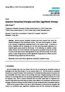
Fig. 3. Iterations Vs. q
Figure 1 (c), (d) show the results of the MAPE and accelerated MAPE algorithm corresponding to maximum SNR. Figures 2 (a), (b), show the variation of SNR, RMSE versus iterations for MAPE and accelerated MAPE algorithm. It is observed that the accelerated MAPE algorithm has faster increase in SNR and faster decrease in RMSE in comparison of conventional MAPE algorithm. Figure 3 shows the variation of exponent q versus iteration number.
5. Conclusion We have given a new method to accelerate the conventional MAPE algorithm. This method adaptively computes exponent of correction term in each iteration using the first-order derivative of the restored image in previous two iteration. From experiment, it is found that accelerated MAPE algorithm gives better results in terms of RMSE, high SNR, in 46% lesser iterations than the conventional MAPE algorithm. While computations required per iteration in MAPE as well as accelerated MAPE algorithms are almost same. This adaptive acceleration method has simple form and can be very easily implemented. Accelerated MAPE algorithm automatically preserves the non-negativity and flux, without additional computations.
220
Manoj Kumar Singh et al.
Acknowledgement This work was supported by the Dual Use Center through the contract at Gwangju Institute of Science and Technology and by the BK21 program in Republic of Korea.
References 1.
Jansson P. A.: Deconvolution of Images and Spectra. New York: Academic Press; (1997)
2. 3.
Katsaggelos A.K.: Digital Image Restoration. New York: Springer-Verlag (1989) A.K. Jain. Fundamental of Digital Image Processing. Engelwood Cliffs, NJ: PrenticeHall (1989) Stark J.L., Murtagh F., Querre P., Bonnarel F.: Entropy and astronomical data analysis. Perspectives from multiresolution. A & A 368, 730–746 (2001) W. H. Richardson. Bayesian-based iterative method of image restoration. J. Opt. Soc. Amer. 62(1), 55–59 (1972) Lucy L. B. : An iterative techniques for the rectification of observed distributions. Astronom. J. 79(6), 745–754 (1974) Meinel E. S. : Origins of linear and nonlinear recursive restoration algorithms. J. Opt. Soc. Amer. A 3(6), 787–799 (1986) Meinel E. S.: Maximum entropy imaage restoration. J. Opt. Soc. Amer. A 5(1), 25–29. (1988) Biggs D.S.C., Andrews M.: Acceleration of Iterative image restoration algorithms. Applied Optics 36(8),1766–1775 (1997) Nunez J., Llacer J. : A fast Bayesian reconstruction algorithm for emission tomography with entropy prior converging to feasible images. IEEE Trans. on Med. Imaging 1990; 9( 2), 159–171 (1990) Nikolova M. :Local strong homoginity of a regularized estimator. SIAM J. Appl. Math. 61, 3437–3450 (2000). Dias J. : Bayesian Wavelet based image deconvolution: A GEM algorithm exploiting a class of heavy– tailed priors. IEEE Trans Image Process 15( 4), 937–951 (2006). Zhou Z., Leahy M., Qi J. : Approximate maximum likelihood hyperparameter estimation for Gibbs priors. IEEE Trans Image Process 6(6), 844–861 (1997) Katkovnic V., Egiazarian K., Astola J.: Local approximation techniques in signal and image processing. Bellingham, Washingtoon: SPIE press (2006)
4. 5. 6. 7. 8. 9. 10. 11. 12. 13. 14.