Adaptive Quantization Using Piecewise Companding and Scaling ...

Adaptive Quantization Using Piecewise Companding and Scaling for Gaussian Mixture Lei Yang and Dapeng Wu [email protected], [email protected] Department of Electrical and Computer Engineering, University of Florida, Gainesville, FL

Abstract Quantization is fundamental to analog-to-digital converter (ADC) and signal compression. In this paper, we propose an adaptive quantizer with piecewise companding and scaling for signals of Gaussian mixture model (GMM). Our adaptive quantizer operates under three modes, each of which corresponds to different types of GMM. Moreover, we propose a reconfigurable architecture to implement our adaptive quantizer in an ADC. We also use it to quantize images and design the tone mapping algorithm for high dynamic range (HDR) image compression. Our experimental results show that 1) the proposed quantizer is able to achieve performance close to the optimal quantizer (i.e., Lloyd-Max quantizer for GMM) in the sense of Mean Squared Error (MSE), at much lower computational cost than it; 2) the proposed quantizer is able to achieve much better MSE performance than a uniform quantizer, at a cost similar to the uniform quantizer. The proposed adaptive quantizer holds great potential in the appilcations of the existing ADC and HDR image compression. Keywords: Scalar quantization, Companding, Scaling, Lloyd-Max quantizer, Gaussian mixture model (GMM), Analog-to-digital converter (ADC), High dynamic range (HDR) image, Tone mapping 1. Introduction Quantization is a critical technique for analog-to-digital conversion and signal compression. On one hand, many input signals are continuous analog signals, therefore, quantization is indispensable for analog-to-digital converters (ADC) [1], which are important components of many digital products. On the other hand, Preprint submitted to Visual Communication and Image Representation

June 9, 2012

with the exponential growth of usage of computers and Internet, countless digital contents, especially digital images and videos, demand signal compression for efficient storage and transmission. Accordingly, quantization provides a means to represent signals efficiently with acceptable fidelity for signal compression. Existing quantization schemes can be classified into two categories, namely, uniform quantization and nonuniform quantization [2, 3]. Uniform quantization is simple, but not optimal for signals with nonuniform distribution in terms of MMSE if more computations and storage are available. While nonuniform quantization is much more complex and in a great variety. Minimum mean squared error (MMSE) quantization (a.k.a, Lloyd-Max quantization) is a major type of nonuniform quantization. It is optimal in the sense of mean squared error (MSE), but incurs high computational complexity. Companding, which consists of nonlinear transformation and uniform quantization, is a technique capable of trading off quantization performance with complexity for nonuniform quantization. Especially, for high rate compression, the performance of companding can approach that of Lloyd-Max quantization asymptotically. Lloyd-Max quantizers and companders are already well developed for Gaussian distribution or Laplacian distribution [2, 4, 5] as convenience, but not for Gaussian mixture model (GMM). Since GMM serves as a good approximation of an arbitrary distribution, it is important to develop quantizers and companders for GMM, which are expected to find wide applications in ADC and high dynamic range (HDR) image compression, as well as audio [6] and video [7] compression. To address this, we proposes a succinct adaptive quantizer with piecewise companding and scaling for GMM in this paper. We first consider a simple GMM (SGMM) that consists of two Gaussian components with mean −µ and µ respectively, and the same variance σ 2 . The proposed quantizers have three modes, making them capable of adapting their reconstructed levels to the varying means and variances of the Gaussian components in a GMM. Specifically, for SGMMs, if µ is small, our quantizer operates in Mode I, and treats the input as if it were from two overlapping Gaussian random variables (r.v.) rather than a GMM r.v.. For Mode I, our quantizer can be implemented by a compander or a scaled Lloyd-Max quantizer of a unit-variance Gaussian. If µ is large, our quantizer operates in Mode III, i.e., if the input is negative, treat the input as if it were a Gaussian r.v. with mean −µ; if the input is positive, treat the input as if it were a Gaussian r.v. with mean µ. For Mode III, our quantizer can be implemented by two companders or two scaled Lloyd-Max quantizers, each of which corresponds to one of the two Gaussian r.v.s. If µ is of medium value, our quantizer operates in Mode II, i.e., with piecewise companding. 2

Moreover, we propose a reconfigurable architecture to implement our adaptive quantizer in an ADC. The proposed adaptive quantizer is tuned by the information from a signal histogram estimator to optimally quantize signals with available speed and power from devices. Furthermore, the proposed quantizer is applied into image quantization and high dynamic range image compression. We design HDR tone mapping algorithm by jointly using adaptive quantizers and multiscale techniques. Therefore, the proposed algorithm could mitigate the halo artifacts in the resulted low dynamic range image, as well as keep the contrast of image details crossing the largest gamut. The experimental results show that 1) our proposed quantizer is able to achieve MSE performance close to Lloyd-Max quantizer for GMM, at much lower cost than Lloyd-Max quantizer for GMM; 2) our proposed quantizer is able to achieve much better MSE performance than a uniform quantizer, at a cost similar to the uniform quantizer. The experimental results also show that the proposed adaptive quantizer holds great potential in the applications of ADC and HDR image compression. It works well with both high rate and low rate quantization. The rest of the paper is organized as below. Section 2 presents the preliminaries of optimal adaptive quantizers. Section 3 describes the proposed adaptive quantizer for GMM. In Section 4, we propose a reconfigurable architecture to implement our adaptive quantizer in an ADC. In section 5, the proposed quantizer is applied into high dynamic range image compression. Experimental results are exhibited in Section 6. Section 7 concludes the paper. 2. Preliminaries of Adaptive Quantizer 2.1. MMSE Quantizer The performance of a quantizer can be evaluated by mean square error (MSE) ˆ i.e., between input signal X and the reconstructed signal X, ˆ 2] MSE = E[(X − X)

(1)

Lloyd-Max quantizer [8] is an MMSE quantizer. Let tk (k = 0, · · · , N) denote boundary points of quantization intervals, and let rk (k = 0, · · · , N − 1) denote quantization levels. Then Lloyd-Max quantizer is characterized by:

3

{t∗k , rk∗ } = arg min MSE {tk ,rk }

= arg min

{tk ,rk }

N −1 Z tk+1 X tk

k=0

(x − rk )2 fX (x)dx

(2)

where fX (x) is the probability density function (pdf) of X, N is the number of quantization levels. Deriving respect to tk and rk in Eq. 2, we have the centroid and the nearest neighbor conditions as following: t∗k = and

∗ rk−1 + rk∗ , 2

k = 1, · · · , N − 1,

R t∗k+1

xp(x)dx t∗ rk∗ = Rkt∗ , k+1 p(x)dx ∗ t

k = 0, · · · , N − 1,

(3)

(4)

k

[t∗0 , t∗N ]

where is the range of the quantizer input. The Lloyd-Max quantizer for Gaussian distribution with zero mean and unit variance has been well studied. Given the number of quantization levels N, the Lloyd-Max quantizer for zero mean, unit variance Gaussian could be obtained from tables in [4]. Given the Lloyd-Max quantizer for zero mean, unit variance Gaussian, we can use the affine law in Proposition 1 to obtain the Lloyd-Max quantizer for Gaussian distribution with arbitrary mean µ and arbitrary variance σ2. 2.2. Gaussian Mixture Model and Affine Law Gaussian distribution is wildly used in signal modeling because of its simplicity, ubiquity, and the Central Limit Theorem. However, signals in the real world, such as pixel intensity of natural images, may have an arbitrary distribution, which can be better approximated by a GMM than by a Gaussian distribution. The pdf of a GMM r.v. X is given as below: fX (x) =

Ng X i=1

pi · gi (x)

(5)

where Ng is the number of Gaussian components in the GMM; gi (x) is the Gaussian pdf for component i (i = 1, · · · , Ng ); pi denotes the probability of component 4

PNg i (i = 1, · · · , Ng ); and i=1 pi = 1. In this paper, we firstly consider a Simple GMM (SGMM) given as below: 1 1 1 2 2 fX (x) = √ (e− 2 (x−µ) + e− 2 (x+µ) ) 2 2π

(6)

Given a suboptimal quantizer for SGMM, we can use the affine law in Proposition 1 to obtain a suboptimal quantizer for a GMM that consists of two Gaussian components with arbitrary mean −µ and µ (µ > 0), respectively and the same variance σ 2 (σ 2 > 0). It can also be used to obtain the suboptimal quantizer for a GMM with arbitrary number of components. Proposition 1. (Affine Law) For a r.v. X with zero mean and unit variance, assume that its N-level Lloyd-Max quantizer is specified by tk (k = 0, · · · , N) and rk (k = 0, · · · , N − 1). Then for r.v. Y = σX + µ, with mean µ and variance σ, its Lloyd-Max quantizer is specified by tˆk = σtk + µ (k = 0, · · · , N) and rˆk = σrk + µ (k = 0, · · · , N − 1). 2.3. MMSE Compander A compander consists of a compressor, a uniform quantizer, and an expandor; the compressor performs nonlinear transformation and the expandor is an inverse of the compressor. The compressor is intended to convert the input r.v. of arbitrary distribution into a uniformly-distributed r.v., so that we can use a simple uniform quantizer, which is the optimal quantizer for the one-dimensional uniform distribution in the sense of MMSE. Proposition 2 gives a nonlinear transformation for an (suboptimal) MMSE compander for any distribution. Proposition 2. Assume that a r.v. X has Cumulative Distribution Function (CDF) FX (x) (x ∈ R). Then r.v. Y = FX (X) is uniformly distributed in [0, 1]; and the compander with compressor Y = FX (X) is an optimal/suboptimal MMSE quantizer of X, especially when X is quantized with high rate. For Gaussian distribution with zero mean and unit variance, a MMSE compressor performs transformation by 1 − Q(X), where Z ∞ 1 u2 Q(X) = √ (7) exp(− )du. 2 2π X Since the integral in Q(X) has high computational complexity, in this paper, we propose a simple compressor, which only needs computation of piecewise monomials (see Section 3.4). 5

3. Adaptive Quantizer for Gaussian Mixture Models In this section, we first present our adaptive quantizer for SGMM in Eq. (6) and then extend it to a more complicated GMM with arbitrary µ and σ 2 , and arbitrary number of components, by using Proposition 1. 3.1. Design Methodology Because Proposition 2 states that the compander with compressor Y = FX (X) is a MMSE quantizer of input X, our design methodology is to find a compressor whose transformation function is simple, but can achieve a good approximation of CDF FX (X). The robust quantizer [9] will be provided through the determination of the required parameters.

Figure 1: CDF of Gaussian N (0, 1) vs. CDF of SGMM with µ = 0.5.

Figure 2: Transformation function of a piecewise compressor vs. CDF of SGMM with µ = 1.5.

Fig. 1 shows the CDF of Gaussian N(0, 1) vs. that of SGMM with µ = 0.5. We can observe that they are similar. Fig. 2 shows the transformation function of a piecewise compressor specified by Eq. (10) vs. CDF of SGMM with µ = 1.5. From Fig. 2, we could observe that the transformation function of a piecewise compressor specified by Eq. (10) is similar to the CDF of SGMM with µ = 1.5. 6

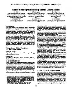
Figure 3: CDF of the catenated Gaussian vs. CDF of SGMM with µ = 3.

Fig. 3 shows two catenated CDFs of two Gaussians vs. the CDF of SGMM with µ = 3, where the catenated CDF of two Gaussians is given by Eq. (16). From Fig. 3, it is observed that the CDF of the catenated Gaussian is similar to the CDF of SGMM with µ = 3. For this reason, our proposed adaptive quantizer operates under three modes, which correspond to small µ, medium-valued µ, and large µ, respectively. 3.2. Three Modes Let qg (X) denote the Lloyd-Max quantization function for a Gaussian r.v. X ∼ N(0, 1). Our proposed adaptive quantizer operates in one of the following three modes, depending on the value of µ. 1. If 0 ≤ µ < µS , the quantizer operates in Mode I, i.e., the quantizer can be an MMSE compander for Gaussian N(0, 1), or Lloyd-Max quantizer for Gaussian N(0, 1). Denote the quantization function in Mode I by qI (X). We use Lloyd-Max quantizer for Gaussian N(0, 1) to implement Mode I, i.e., qI (X) = qg (X). (8) The motivation of using Mode I is that the CDF of Gaussian N(0, 1) is similar to the CDF of SGMM with small µ as shown in Fig. 1. 2. If µS ≤ µ < µL , the quantizer operates in Mode II, i.e., the quantizer is a compander with a piecewise compressor specified by Eq. (10). The motivation of using Mode II is that the transformation function of a piecewise compressor specified by Eq. (10) is similar to the CDF of SGMM with medium-valued µ as shown in Fig. 2.

7

3. If µ ≥ µL , the quantizer operates in Mode III, i.e., the quantizer can be two catenated MMSE compander for two Gaussians, or two catenated LloydMax quantizers for two Gaussians. Denote the quantization function in Mode III by qIII (X). We choose the catenated Lloyd-Max quantizer to implement Mode III as following: ( qg (X − µ) , X ≥ 0 (9) qIII (X) = qg (X + µ) , X < 0 The motivation of using Mode III is that two catenated CDFs of Gaussian is similar to that of SGMM with large µ as shown in Fig. 3. 3.3. Parameter Determination In this section, the values of µS and µL will be determined. It is well known the 3-sigma rule that nearly all (99.7%) of the values lie within 3 standard deviations around the mean for Gaussian distribution. Therefore, if µ ≥ 3, the two Gaussian components of SGMM could be dealt with respectively, as in Mode III. When µ < σ, for SGMM, the data of right Gaussian component in [µ − σ, µ + σ], always fall in the [−µ − 3σ, −µ + 3σ], the 3 standard deviations around the mean of left Gaussian component, and vise versa. Therefore, for σ = 1, when 0 ≤ µ < 1, we consider the data of SGMM as Mode I. In conclusion, for the proposed quantizer µS = 1 and µL = 3. 3.4. Piecewise Companding of Mode II For Mode II, we choose the monomial f (x) = axb to approximate the ideal compressor of SGMM, i.e. the CDF of SGMM, piecewisely. There are many more accurate and P more complicated approximative functions, like the sum of monomials f (x) = i ai xbi , i > 1, sigmoid function f (x) = 1+e1−x , and f (x) = arctan(x). But their corresponding expandors, i.e. the inverses of compressors, are hard to obtain or computationally expensive. However, f (x) = axb has simple inverse and is a good approximation to the segments of the CDF of SGMM. The piecewise compressor symmetrical to the origin can be described by Eq. (10).  a(x + µ)b + 0.25, x ≤ −µ     a′ (x + µ)b′ + 0.25, −µ < x ≤ 0 f (x) = ′  −a′ (µ − x)b + 0.75, 0 < x ≤ µ    a(x − µ)b + 0.75, x > µ 8

(10a) (10b) (10c) (10d)

with {a, a′ , b, b′ } = arg Z 3 Z min ( ′ ′ {a,a ,b,b }

1

∞

−∞

(FSGM M (x, µ) − f (x, µ))2 dx)dµ

(11)

By the steepest descent method, we obtain b = 31 , b′ = 21 , a = 0.15 and a′ = 0.125 (which can be realized by right shifting 3 bits) for simplicity and fast computation. The compressor is shown in Fig. 2 when µ = 1.5. When x < −µ and x > µ, 1 the PDF decaying faster, we use f (x) = ax 3 . When x > −µ and x < µ, the 1 PDF decaying slower, we use f (x) = a′ x 2 . It results that the data with small probability is compressed more and the data with large probability is compressed less. It is more precise than piecewise linear compander [9], and still simple. Although there are more accurate compressors to approximate the CDF with certain µ, they may not have good approximations to the CDF with other µ ∈ [1, 3) in average. The proposed compressor is a good tradeoff between accuracy and generalizability. It provides a stable good performance when µ ∈ [1, 3) as shown in experiments in Section 6. It is robust.

Analog Signal x(t)

Discrete Signal x[n]

Uniform Quantizer

Inverse Uniform Quantizer

Histogram Estimation

Sampling and Hold Circuit FPGA Adaptive Quantizer

Figure 4: Reconfigurable A/D converter.

Therefore, the proposed compander has three advantages. 1. It is easy to design compander by Eq. (10); 2. It is fast to quantize data with this compander; 3. It has good average MSE performance when µ ∈ [1, 3). 3.5. Adaptive Quantizer for A General GMM In this section, we design the adaptive quantizer for a general GMM based on the adaptive quantizer for SGMM. 9

3.5.1. GMM Estimation by EM The GMM (Gaussian Mixture Model) is a probability distribution model consisting finite number of Gaussian components as shown in Eq. (5). The ExpectationMaximum (EM) algorithm [10] is a general method to find the maximum likelihood estimation of GMM. −3

9

x 10

Original Histogram Gaussian Component 1 Gaussian Component 2 Gaussian Component 3 Gaussian Component 4 GMM Estimation

8 7

Pixel Frequency

6 5 4 3 2 1 0

0

50

100 150 Pixel Value

200

250

Figure 5: GMM estimation by EM algorithm on histogram of Barbara.

EM algorithm can efficiently estimate the components of GMM [11] as shown in Fig. 5. The number of components of GMM should be assigned to the EM algorithm by experience and restricted by the available computational resources and N, the number of the reconstruction levels of quantizers. Ng could be N/5 or smaller. µi , σi and pi (i = 1, · · · , Ng ) of each Gaussian component in Eq. (5) are determined by the EM algorithm. The GMM estimation of signals with stable distribution is obtained for later quantization once for all. 3.5.2. Generalization by Processing Neighboring Gaussian Components Pairwisely For the General GMM as shown in Eq. (5), with the scaling law in Proposition 1, the following generalizations are made from SGMM by considering neighboring pairwise Gaussian components. Assuming the Gaussian components are sorted by their means µi , for the neighboring Gaussian components Ci and Ci+1 , we consider support (µi , µi+1 ), when i 6= 1, Ng , else consider (−∞, µ1 ) or (µNg , +∞). 1. Allocate the number Ni from the total reconstruction levels N for each 10

Gaussian component according to its percentage pi . Ni = [N · pi ] where [·] is round off operator. For each Ni , it is symmetrically located with respect to the mean of the corresponding Gaussian component. 2. Origin Shift: For any two adjacent Gaussian components with means and variances of 2 (µi , σi2 ) and (µi+1 , σi+1 ), their pdfs equal around xo =

σi µi + σi+1 µi+1 σi + σi+1

(the effect of pi is omitted). Then we shift the origin to xo . 3. The three-mode boundaries µS and µL are scaled by (σi + σi+1 ). 4. Scale the reconstruction levels according to the variance: For the Gaussian component i with (µi , σi ), scale the reconstruction levels obtained from SGMM by σi . 5. Tune mode II: Since half support (µi , µi+1 ) of Gaussian components is considered each time, the compressor in Eq. (10b) (10c) are needed, and should be scaled by pi as: ( ′ pi (a′ (x + µ)b + 0.25), −µ < x ≤ 0 f (x) = (12) ′ pi (a′ (x + µ)b + 0.25), −µ < x ≤ 0 In this way, the adaptive quantizer for a GMM is determined. 4. Reconfigurable A/D converter with Adaptive Quantizer With the proliferation of autonomous sensors, and digital devices, there has been an increasing demand for reconfigurable analog-to-digital converters (ADC) [12], where the proposed adaptive quantizer can have important applications. We propose a reconfigurable A/D converter adaptive to the distribution of the input signals with the proposed quantizer as shown in Fig. 4. For the input signal with arbitrary distribution, we quickly sample and discretize it with uniform quantizer to estimate the distribution of the signal. This information is sent back to the proposed adaptive quantizer to do mode selection. Then the adaptive quantizer could give a more accurate discrete signal by capturing the signal characteristics as much as possible with appropriate modes. The residual signal could also be 11

iteratively sent back to the adaptive quantizer to minimize the quantization error. The FPGA implementation of the adaptive quantizer could be reconfigured in Tq milliseconds, where Tq < 10. Then the system can be updated at the beginning of every cycle of Tq milliseconds, according to the distribution of the input signal. The number of quantization levels could be adjusted according to the speed, resolution and power consumption of the devices. Our scheme based on histogram estimation and the GMM modeling may outstand previous iterative DPCM schemes [13]. The reconfigurable ADC architecture in Fig. 4 can dynamically adjust the quantization speed, resolution and power consumption to match input data characteristics. Therefore, it will have wide applications in many ADCs and sensor applications. 5. High Dynamic Range Image Compression with Joint Adaptive Quantizer and Multiscale Techniques High dynamic range imaging (HDRI or just HDR) is one of the frontier techniques in image processing, computer graphics and photography [14, 15, 16], where image pixels take floating values in the range of [0,1] rather than the traditional 8 bits per pixel for gray images and 24 bits per pixel for RGB images. HDRI try to capture the dynamic range of natural scenes, which can exceed three orders of magnitudes of display devices. The dynamic range of natural scenes can be captured by human eyes, many films, and new camera sensors. Whereas, display devices, such as CRTs, LCDs, and print materials, are restricted to low dynamic range. Therefore, compressing the high dynamic range of HDRI to adapt to the low dynamic range of display devices and keeping the vivid colors and the rich details of the original images as much as possible, is getting more and more attention. It is called tone mapping, which is an important component in the HDR imaging pipeline, and widely used in virtual reality, video advertising, visual simulation, remote sensing images, aerospace, medical and many other fields [17]. The tone mapping techniques can be divided into two categories: tone reproduction curves (TRCs) and tone reproduction operators (TROs). They could be applied to images both globally and locally. TRCs use compressive point nonlinearity mapping, such as a power function f (·), to shrink the high dynamic range images into the low dynamic range images. K. Chiu et al. proposed spatially nonuniform scaling functions for high contrast images [18]. F. Drago et al. used an adaptive logrithmic mapping for displaying high contrast scenes [19]. Erik Reinhard et al. [20] developed their tone mapping method based on the well12

known photo-graphic pratice of dodging-and-burning. Fattal et al. [21] manipulate scale factors in the gradient domain of logarithmic space. Larson et al. [22] proposed a histogram adjustment technique adaptive to the luminance in the scene. I.R. Khan et al. [23] and A. Boschetti et al. [24] improved the histogram based algorithms by incorporating human visual system, and adjusting the histogram locally. Jiang Duan et al. [25] neatly combined the global tone mapping operator HALEQ into local tone mapping operator ALHA, with fixed parameter values and good performance. Also they proposed several algorithms [26, 27] for compressing HDRI by optimally combining linear map and histogram equalization. The TROs adjust pixel intensity by using spacial context to preserve local image contrast, which usually use multiscale techniques. Stockham [28] separated an HDR image H(x, y) into a product of an illumination image I(x, y) and a reflectance image R(x, y) in an early literature. Later on, Jobson et. al. [29], Pattanaik et.al [30] improved the multiscale techniques by introducing mechanism of the human visual system. Later Frdo Durand and Julie Dorsey [31] presented a new technique with fast bilateral filtering decompositing images into a base layer, and a detail layer. These multiscale methods have halo artifacts, which happen around the sharp edges and are caused by the blurring effect of filters. The most recent multiscale technique proposed by Yuanzhen Li [32] properly used a symmetric analysis-synthesis filter bank, and local gain control of each subband to mitigate the halo artifacts. But the luminance of the resulted low dynamic range images seems low, and the boundary of the dynamic range is clipped, which could be seen from their histograms. To address these problems, we proposed a joint TRC and TRO methods for high dynamic range image tone mapping based on Li’s method [32] and our proposed adaptive quantizer. We proposed two methods to use the proposed adaptive quantizer for HDRI tone mapping. The first method is shown in Fig. 6. Adaptive quantization is taken in the log domain of pixel values. And then in each quantization range, linear mapping is used to map vaues into target LDR values as shown in Eq. (13) for 8-bit per pixel output. f (x) =

256 x − tk ( + k), k = 0, · · · , N − 1. N tk+1 − tk

(13)

where N(1 ≤ N ≤ 256) is the number of quantization levels, [tk , tk+1 ] is the kth quantization range. The adaptive quantization acts as histogram equalization, to maximize image contrast. Linear mapping tries to keep the perceptual feeling of N is an indicator of balance between adaptive quantithe original images. q = 256 13

zation and linear mapping. If q = 1, no linear mapping is involved in HDRI tone 1 mapping. If q = 256 , no adaptive quantization is involved in HDRI tone mapping.

Figure 6: Tone mapping by using joint adaptive quantizer and linear mapping.

The second method is to use the adaptive quantizer in the post processing of HDR images as shown in Fig. 7. After adaptive quantization, the LDRI has more uniform constrast in the full low dynamic range of LDRI obtained from TRO methods.

Figure 7: Tone mapping by using joint adaptive quantizer and multiscale techniques.

6. Experimental Results and Discussion We compare the proposed quantizer with the actual Lloyd-Max quantizers for SGMM, by comparing the corresponding approximate CDFs of the proposed

14

quantizer with the actual CDFs of SGMM. We also compare the proposed quantizer with the Lloyd-Max quantizers for SGMM and the uniform quantizer in terms of MSE performance. The proposed adaptive quantizer is described in detail in Section 3. The LloydMax quantizer for SGMM is found by the LBG algorithm numerically [2]. The uniform quantizer we compare with is the optimal uniform quantizer which is applied uniformly to the finite region containing 99.8% of the data of the GMM distribution. 6.1. Example and Justification of Parameter Determination The reproduction values of 2-bit Lloyd-Max quantizer for N(0, 1) are [−1.5104, − 0.4528, 0.4528, 1.5104]. When µ ≥ 3, for the 3-bit quantizer for SGMM, the 8 reproduction values are [−1.5104 − µ, − 0.4528 − µ, 0.4528 − µ, 1.5104 − µ, − 1.5104 + µ, − 0.4528 + µ, 0.4528 + µ, 1.5104 + µ] as in Mode III. When µ < 1, i.e. in mode I, for the 2-bit quantizer for SGMM, the reproduction values are [−1.5104, − 0.4528, 0.4528, 1.5104]. When 1 ≤ µ < 3, i.e. in mode II, the compander is chosen as shown in Eq. (10). The differences between reproduction values of the proposed quantizer and those of the Lloyd-Max quantizer for SGMM are evaluated by average absolute difference (AAD) as following: AAD =

Z

c

d

N −1 1 X p |r (µ) − rkl (µ)|dµ N k=0 k

(14)

where rkp and rkl are the reproduction values of the proposed quantizer and the Lloyd-Max quantizer for SGMM, µ is the mean in SGMM, (c, d) is the support for averaging, i.e. the region of µ for each mode. The approximation error between the CDF approximators in the proposed quantizer and those of SGMM is evaluated by: Z d Z ∞ ( (FSGM M (x, µ) − FA (x, µ))2 dx)dµ (15) c

−∞

where FSGM M is the CDF of SGMM, FA is the CDF approximators in the proposed quantizer. For Mode I, c = 0, d = 1, FA (x) = Q(x) where Q(x) is defined

15

Table 1: Proposed Quantizer vs. Lloyd-Max quantizer.

Mode I Mode II AAD 10−2 10−1 Approximation Error 2.51 16.69

Mode III 10−4 0.03

Table 2: Comparison of Complexity of Quantizaters.

Quantizers Uniform Quantizers Mode I qI (x) Proposed Companding Adaptive Mode II Quantizer Mode III qIII (x) Companding Lloyd-Max Quantizer for GMM

Design Time Inv N N N N/2 N 2k · N ·(Int+1)

Running Time per Sample 3 logN 4 4 log(N/2) 4 logN

Memory O(1) O(N ) O(1) O(1) O(N ) O(1) O(N )

(N is the number of quantization levels; Inv denotes the complexity of computing the inverse of CDF; Int denotes the complexity of computing the integral, k is the number of iterations in Lloyd-Max algorithm.)

in Eq. (7); for Mode II, c = 1, d = 3, FA (x) is in Eq. (10); for Mode III, ( (1 + Q(x + µ))/2, x 0 on the support. By using Bennettt’s [35] approximate expression for the mean

25

square distortion for very large number N of quantizer output levels, we have: Z b 1 1 2 ˆ ]∼ E[(X − X) dx (B.2) = 12N 2 a fX (x) It is bounded by

1 1 (b − a) max { } (a,b) fX (x) 12N 2

Therefore, Eq. (B.2) is towards 0 as N → ∞. References [1] Johns, D., Martin, K.. Analog integrated circuit design. Wiley India Pvt. Ltd.; 2008. [2] Gray, R.M., Neuhoff, D.L.. Quantization. IEEE Transactions on Information Theory 1998;44(6):2325–2383. [3] Graf, S., Luschgy, H.. Foundations of quantization for probability distributions. Springer-Verlag New York, Inc. Secaucus, NJ, USA; 2000. [4] Jain, A.. Fundamentals of digital image processing. Prentice-Hall, Inc. Upper Saddle River, NJ, USA; 1989. [5] Peri´c, Z., Milanovi´c, O., Jovanovi´c, A.. Optimal companding vector quantization for circularly symmetric sources. Information Sciences 2008;178(22):4375–4381. [6] Pohlmann, K.. Principles of digital audio. McGraw-Hill/TAB Electronics; 2005. [7] Wiegand, T., Sullivan, G., Bjontegaard, G., Luthra, A.. Overview of the H. 264/AVC video coding standard. IEEE Transactions on Circuits and Systems for Video Technology 2003;13(7):560–576. [8] Gersho, A., Gray, R.. Vector quantization and signal compression. Kluwer; 1993. [9] Kazakos, D., Makki, S.. Piecewise linear companders are robust. In: Proceedings of the 12th Biennial IEEE Conference on Electromagnetic Field Computation 2006. IEEE. ISBN 1424403200; 2006, p. 462–462. 26

[10] Bishop, C., service), S.O.. Pattern recognition and machine learning; vol. 4. Springer New York; 2006. [11] Xuan, G., Zhang, W., Chai, P.. EM algorithms of Gaussian mixture model and hidden Markov model. In: Proceedings of International Conference on Image Processing, 2001.; vol. 1. IEEE. ISBN 0780367251; 2002, p. 145– 148. [12] Gulati, K., Lee, H.. A low-power reconfigurable analog-to-digital converter. IEEE Journal of Solid-State Circuits 2001;36(12):1900–1911. [13] Choi, M., Abidi, A.. A 6-b 1.3-Gsample/s A/D converter in 0.35-µm CMOS. IEEE Journal of Solid-State Circuits 2001;36(12):1847–1858. [14] Debevec, P., Malik, J.. Recovering high dynamic range radiance maps from photographs. In: ACM SIGGRAPH 2008 classes. ACM; 2008, p. 1–10. [15] DiCarlo, J., Wandell, B.. Rendering high dynamic range images. In: Proceedings of the SPIE: Image Sensors; vol. 3965. Citeseer; 2000, p. 392– 401. [16] Devlin, K., Chalmers, A., Wilkie, A., Purgathofer, W.. Tone reproduction and physically based spectral rendering. Eurographics 2002: State of the Art Reports 2002;:101–123. [17] Debevec, P., McMillan, L.. Image-based modeling, rendering, and lighting. IEEE Journal of Computer Graphics and Applications 2002;22(2):24–25. [18] Chiu, K., Herf, M., Shirley, P., Swamy, S., Wang, C., Zimmerman, K.. Spatially nonuniform scaling functions for high contrast images. In: Graphics interface. Citeseer; 1993, p. 245–245. [19] Drago, F., Myszkowski, K., Annen, T., Chiba, N.. Adaptive logarithmic mapping for displaying high contrast scenes. In: Computer Graphics Forum; vol. 22. Wiley Online Library; 2003, p. 419–426. [20] Reinhard, E., Stark, M., Shirley, P., Ferwerda, J.. Photographic tone reproduction for digital images. In: IN: PROC. OF SIGGRAPH02. ACM Press; 2002, p. 267–276.

27

[21] Fattal, R., Lischinski, D., Werman, M.. Gradient domain high dynamic range compression. ACM Trans Graph 2002;21:249–256. doi:\bibinfo{doi} {http://doi.acm.org/10.1145/566654.566573}. URL http://doi.acm. org/10.1145/566654.566573. [22] Larson, G.W., Rushmeier, H.E., Piatko, C.D.. A visibility matching tone reproduction operator for high dynamic range scenes. IEEE Trans Vis Comput Graph 1997;3(4):291–306. [23] Khan, I., Huang, Z., Farbiz, F., Manders, C.. HDR image tone mapping using histogram adjustment adapted to human visual system. In: Proceedings of the 7th International Conference on Information, Communications and Signal Processing 2009. IEEE; 2009, p. 1–5. [24] Boschetti, A., Adami, N., Leonardi, R., Okuda, M.. High Dynamic Range image tone mapping based on local Histogram Equalization. In: Proceedings of IEEE International Conference on Multimedia and Expo (ICME) 2010. IEEE; 2010, p. 1130–1135. [25] Duan, J., Bressan, M., Dance, C., Qiu, G.. Tone-mapping high dynamic range images by novel histogram adjustment. Pattern Recognition 2010;43(5):1847–1862. [26] Qiu, G., Duan, J.. An optimal tone reproduction curve operator for the display of high dynamic range images. In: Circuits and Systems, 2005. ISCAS 2005. IEEE International Symposium on. IEEE; 2005, p. 6276–6279. [27] Qiu, G., Guan, J., Duan, J., Chen, M.. Tone mapping for hdr image using optimization a new closed form solution. In: Pattern Recognition, 2006. ICPR 2006. 18th International Conference on; vol. 1. IEEE; 2006, p. 996–999. [28] Stockham, T.. Image processing in the context of a visual model. Proceedings of the IEEE 1972;60(7):828–842. [29] Jobson, D., Rahman, Z., Woodell, G.. A multiscale retinex for bridging the gap between color images and the human observation of scenes. IEEE Transactions on Image Processing 1997;6(7):965–976.

28

[30] Pattanaik, S., Ferwerda, J., Fairchild, M., Greenberg, D.. A multiscale model of adaptation and spatial vision for realistic image display. In: Proceedings of the 25th Annual Conference on Computer Graphics and Interactive Techniques. ACM. ISBN 0897919998; 1998, p. 287–298. [31] Durand, F., Dorsey, J.. Fast bilateral filtering for the display of highdynamic-range images. In: ACM Transactions on Graphics (TOG); vol. 21. ACM; 2002, p. 257–266. [32] Li, Y., Sharan, L., Adelson, E.. Compressing and companding high dynamic range images with subband architectures. In: ACM Transactions on Graphics (TOG); vol. 24. ACM; 2005, p. 836–844. [33] Hossack, D., Sewell, J.. A robust CMOS compander. IEEE Journal of Solid-State Circuits 1998;33(7):1059–1064. [34] Ma, J., Xu, L., Jordan, M.. Asymptotic convergence rate of the em algorithm for gaussian mixtures. Neural Computation 2000;12(12):2881–2907. [35] Bennett, W.. Spectra of quantized signals. Bell Syst Tech J 1948;27(3):446– 472.

29

(a) E. Reinhard’s method [20]

(b) Histogram based algorithm [23]

(c) Our proposed method 1 (N=128)

(d) Our proposed method 1 (N=64)

Figure 15: Performance comparison between different tone mapping algorithms on HDR image Stanford Memorial Church (copyright by Paul Debevec)

30

(a) E. Reinhard’s method [20]

(b) Histogram based algorithm [23]

(c) Our proposed method 1 (N=128)

(d) Our proposed method 1 (N=64)

Figure 16: Performance comparison between different tone mapping algorithms on HDR image Belgium House (copyright by Raanan Fattal)

31