Adaptive Routing in Underwater Delay Tolerant Sensor Networks

Adaptive Routing in Underwater Delay Tolerant Sensor Networks ∗ Computer

Zheng Guo∗ , Zheng Peng∗ , Bing Wang∗ , Jun-Hong Cui∗ , Jie Wu†

Science and Engineering Department, University of Connecticut, Storrs, CT, 06269 Email: {guozheng, zhengpeng, bing, jcui}@engr.uconn.edu † Computer and Information Sciences Department, Temple University, Philadelphia, PA 19122 Email: [email protected]

Abstract— Underwater Sensor Network (UWSN) has attracted significant attention from both academia and industry. Different from terrestrial sensor nodes, underwater sensor nodes are usually mobile, much bigger, more energy-consuming, harder to recharge and suffer from more severe environmental conditions. Thus, an UWSN can be easily partitioned and no persistent routes from a source to a destination are available. Therefore, an UWSN can be viewed as a Delay/Disruption Tolerant Network (DTN). Moreover, an UWSN is always supposed to work for a long time to accomplish multiple tasks with various application requirements, such as delay and delivery ratio. Although many routing protocols have been proposed for DTNs, they are not suitable for UWSNs and cannot handle various application requirements. In this paper, we propose redundancy based adaptive routing (RBAR) for underwater DTNs. Through analysis and simulation, we demonstrate RBAR can achieve the best energy efficiency while satisfying different delay requirements of various packets by explicitly controlling the replication process.

I. I NTRODUCTION As a promising solution to aquatic environmental monitoring and exploration, Underwater Sensor Network (UWSN) has attracted significant attention recently. Different from terrestrial sensor nodes, underwater sensor nodes are usually mobile, and much bigger, more energy-consuming, harder to recharge and more expensive [1]. Thus, owing to the mobility and sparse deployment, an UWSN can be easily partitioned, with no persistent routes from a source to a destination available. Therefore, an UWSN can be viewed as a Delay/Disruption Tolerant Network (DTN) [2], traditional routing protocols are usually not practical since packets will be dropped when no routes are available. Many routing protocols have been proposed for DTNs. Most of them utilize multiple copies since obviously more copies imply more opportunities to contact the destinations and quicker delivery, such as Epidemic [3], Spray and Wait [4] and PROPHET [5]. These protocols treat all packets equivalently and try to achieve a tradeoff between energy and delay. However, in real scenarios, an UWSN often needs to provide differentiated packet delivery according to various application requirements. For instance, in water pollution monitoring, a packet that reports pollution should be delivered as quickly as possible, while a packet that reports normal conditions (such as conductivity, temperature, and depth) can tolerate a long end-to-end delay. Thus it is desirable to design a smart routing protocol that could handle these different requirements

adaptively. In this paper, we propose redundancy based adaptive routing (RBAR) for underwater DTNs. RBAR allows a node to hold a packet as long as possible until it has to make another copy to satisfy its delay requirement. To achieve this purpose, RBAR adopts a binary tree based forwarding procedure, through which the packet replication process can be explicitly determined. Thus RBAR can achieve the best energy efficiency while satisfying the delay requirements. We also conduct simulations to evaluate the performance of RBAR. The results show that RBAR can adaptively choose the number of copies for packets according to their delay requirements and reach desired delivery ratio for all packets with low energy consumption, while other schemes (such as Epidemic and Spray and Wait) treat all packets equivalently thus cannot achieve the best energy efficiency for all packets. The rest of paper is organized as follows. In Section II, we introduce the related work. Then we describe the network settings and the detailed redundancy based adaptive routing (RBAR) in Sections III and IV. We compare RBAR with other schemes in Section V and conclude our work in Section VI. II. R ELATED W ORK Most DTN routing protocols utilize multiple copies to establish multiple potential paths to the destination. According to the principles of how to replicate multiple copies, we categorize the proposed routing protocols as blind redundancy based routing and utility based routing. A. Blind Redundancy Based Routing Blind redundancy based routing is the most intuitive method for DTNs since increasing the amount of copies also increase the probability that any copy can reach the destination quickly. Epidemic [3] is the first representative multi-copy routing scheme by replicating a packet to any node in the network. It is basically a flooding scheme and can optimize the end-to-end delay by taking every potential route. However, Epidemic is too aggressive to consume the network resources. Aiming to avoid unconstrained replication, Harras et. al. propose several controlled flooding schemes in [6], such as time-to-live, kill time and passive cure. Spyropoulos et. al. present spray and wait [4], in which a predetermined certain number of copies of a packet are replicated to the first encountered nodes.

The schemes above all assume that the source determines the amount of copies disseminated to the network. Actually, it is hard to obtain the network conditions and decide the suitable redundancy in DTNs. Xu et. al. raise adaptive spray mechanisms and let the relays make decisions on the spray depth independently, which can be dynamically adjusted in accordance to the network conditions [7]. These schemes simply disseminate multiple copies to the network to take the advantage of multiple delivery opportunities, thus they do not require any information from the network and incur little overhead. However, these blind replication protocols may consume huge network resources and are not practical for harsh networks, such as underwater DTNs.

are of different importance and have various requirements. The novelty of our work is that we propose a redundancy based adaptive routing protocol, RBAR, using different number of copies according to the characteristics of the packets and the network. III. N ETWORK S ETTING

B. Utility Based Routing Utility based routing is applicable to DTNs, where all nodes in the network have different properties at any time. For example, nodes may prefer different locations (communities) or have various behaviors and routines in social networks [8], [9], [10], while some nodes may have higher contact probability to the destination than others [5]. Therefore, it is possible to design a utility metric reflecting these properties, which is a statistic profile to evaluate the benefits earned from sending a copy to current neighbors. Burgess et. al. propose MaxProp to exploit the priorities based on the path likelihood [11]. Lindgren et. al. present PROPHET [5], in which an intermediate node only forwards a packet to the neighbors who have higher probabilities to reach the packet’s destination in a short time. In [12], Balasubramanian et. al. present an intentional DTN routing protocol, Rapid, to optimize a specific routing metric. Rapid treats DTN routing as a resource allocation problem that translates the targeting metric to per-packet utility and determines the packets replication in the network. In addition, Jones et. al. utilize the contact history to find routes with minimum estimated expected delay [13]. Wu et. al. propose a scheme that forwards packets to relays with increasing utility to increase reliability [14]. The scheme by Cardei et. al. makes routing decisions based on the probabilistic trajectory prediction [15]. Liu et. al. present optimal probabilistic forwarding (OPF) to maximize the expected delivery rate while satisfying a certain constant on the number of forwardings per packet in [16]. In these schemes, utility is determined by either the special network hierarchy or the underlying mobility model. Utilities are different for different nodes, thus replication is possible along the path of increasing utility. Compared with blind redundancy based routing protocols, utility based routing protocols always have better performance regarding to certain criteria, but they also require more information from the network and incur heavy overhead to maintain and calculate the utility. All the DTN routing protocols above, both blind redundancy based routing and utility based routing, treat all packets equally and aim at a single optimization goal, e.g., minimizing average end-to-end delay, maximizing delivery rate or energy efficiency. None of them is suitable for the applications where packets

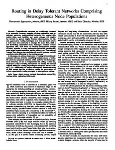
Base station

Fig. 1.

Sink

Sensor

System model.

We consider a UWSN as shown in Figure 1. N sensors are deployed in the bottom of the sea while M buoys float on the surface to collect data generated by the sensors. Both sensors and buoys move following the Random Waypoint model. Thus, for any pair of sensors, the inter-contact time t follows exponential distribution with intensity λ as f (t, λ) = λeλt [17]. This means that the process of the contact between this pair is a poisson process and the number of contacts k within the interval t follows poisson distribution as f (k, λt) = (λt)k eλt . We assume every node-node pairs have the identical k! inter-contact pattern. Similarly, we assume the contact process of node-sink pairs is also a poisson process with intensity µ. The node buffer is assumed to be infinite and no overflow happens, while the bandwidth is high enough to transfer the whole bundle of packets in the buffer during one contact. Since all nodes are identical (homogeneous network) and poisson process is memoryless, for a pair of nodes, the next expected contact always follows the same exponential distribution at any time. Thus, there will be no obvious better relay node for a packet, as some probability based or utility based DTN routing schemes do like PROPHET. With this assumption, the expected delay only relates to the number of nodes who hold this packet, thus the redundancy based routing schemes like Epidemic, Spray and wait will be better choices. We consider the application of water pollution surveillance. Sensor nodes generate packets with different emergency priorities to be delivered to the sinks(buoys), and packets with different priorities can tolerant different delay. To demonstrate that our new scheme can satisfy the application requirements, we assume each packet has an explicit delay requirement associated with its emergency. The emergency level p of a

packet when generated is uniformly randomly selected in the range of [0, 100] and the delay requirement D is D(p) = a×p+b, where a and b are pre-determined. The objective is to guarantee punctual delivery and achieve high energy efficiency at the same time. IV. R EDUNDANCY BASED A DAPTIVE ROUTING In this section, we first introduce the replication procedure, then model it as a continuous Markov chain with absorbing state. With this model, each node can obtain a common replication sequence in a distributed manner. Afterwards, we analytically study the system delay distribution and energy consumption for a packet with any delay requirement.

by the node. The dashed line means a node keeps holding a packet, while the solid lines with time stamps imply that when this node should replicate one copy to another node. If a node holds the ith copy, it is responsible to make the lth copy until time tl , where l = 2(⌈log2 i⌉+j) + i (j = 0, 1, 2, . . . , ⌊log2 N ⌋, l ≤ N ). After replication, the receiving node will record its copy index l and calculate its responsible time stamp to replicate. Any node holding a packet contacts any one sink can forward this packet to the base station through this sink (buoy). Then all sinks (buoys) immediately broadcast an acknowledgement to the network. B. Markov Model

A. Forwarding Procedure In RBAR We adopt a binary tree based forwarding procedure for the copy replication. Spyropoulos et. al. propose a similar scheme, Spray and Wait, to randomly distribute n copies to the network, where n is pre-determined [18]. In RBAR, the number of copies required is varying over time and we want to control the global number of copies in the network at any certain time. Thus, each node should estimate the current number of copies and implicitly cooperate to be aware that which node is responsible to replicate the next copy in a distributed way.

r0,1

S1

r1,2

S2 g1,N+1

r2,3

ri-1,i

Si

g2,N+1

gi,N+1

ri,i+1

rN-1,N

rN,N+1

SN

gN,N+1

SN+1 A

1 A2

A

B

1

2

Fig. 3.

A3

A

C

1 A5

A

1

E

0

A1

Fig. 2.

B

3 A7

5

C

Markov model with absorbing state

A4

3

G

A2

D

2 A6

7

B

A3

2

F

A4

4 A8

D

6

A5

4

A6

H

8

A7

A8

The forwarding procedure of a packet

The essential part of RBAR is allowing a node to hold a packet as long as possible until very necessary to make another copy. Figure 2 shows the forwarding procedure for a certain packet, which is generated at time t0 at node A. Without loss of generality, we assume t0 = 0. We first assume every node is aware that there exist a global time sequence Ai (i = 1, 2, 3, . . . , N ) (The estimation of the time sequence will be described in Section IV-C), which means until the age of the packet until Ai , there should be i copies in the network, otherwise, this packet cannot be delivered to the sinks with high probability. The circles with identifications in Figure 2 represent the nodes which have copies, the numbers besides circles indicate the index of the corresponding copies held

We model the packet replication process as a continuous Markov chain with absorbing state as shown in Figure 3 [19]. We assume all nodes keep replicating copies according to the forwarding procedure as aforementioned in a distributive manner. Thus, we can calculate the necessary time stamps in Figure 2 using this Markov model. In this model, the state Si (1 ≤ i ≤ N ) represents that there are i copies in the network, and the state SN +1 represents the absorbing state, which means this packet is delivered to one of the sinks (buoys). N is the predetermined maximum number of copies allowed in the network, which means at most N nodes will eventually have a copy. In this setting, N is the total number of nodes. The state Si can only transfer to the state Si+1 with rate ri,i+1 or directly transfer to the state SN +1 with rate gi,N +1 . Ideally, the state Si corresponds to the time range [Ai , Ai+1 ]. When the network is in the state Si , there should be i copies in i different nodes. Every node is aware that only one of them is responsible to make a copy to any one node of the left N −i nodes which do not have this copy. Since any pair of nodes has identical contact process following poisson distribution with intensity λ, thus the transfer rate from Si to Si+1 can be obtained as ri,i+1 = (N − i)λ,

1≤i≤N −1

(1)

Similarly, since there are i nodes with copies and M sinks (buoys) and each node-sink pair follows poisson process with intensity µ, we can also get the transfer rate from Si to SN +1 as gi,N +1 = iM µ, 1≤i≤N (2) The rate r0,1 represents there is a packet ready for delivery, thus we have r0,1 = 1. We also have rN,N +1 = 0. We use Fi1 (t)(1 ≤ i ≤ N +1) to denote the probability that the network is in the state Si until time t, starting from the state S1 when the source is ready to replicate the second copy (the original packet is the first copy), which responds to t1 in Figure 2. Without loss of generality, we assume A1 = 0, thus F11 (0) = 1 and Fi1 (0) = 0(2 ≤ i ≤ N +1). According to Kolmogorov’s equation, we can derive the following differential equations about the continuous Markov chain:  dF 1 (t) 1 (t) 1 = −(r1,2 + g1,N +1 )F1    dt ... dFi1 (t) 1 = ri−1,i Fi−1 (t) − (ri,i+1 + gi,N +1 )Fi1 (t) (3) dt  ...   dFN1 +1 (t) ∑N 1 =

dt

    

j=1 gj,N +1 Fj (t)

Applying Laplace transform on equation 3, we can get 1 (s) − F 1 (0) sF1 1

= ...

sF 1 (s) − Fi1 (0) i

= ...

1 sF 1 (s) − FN +1 (0) N +1

=

1 (s) −(r1,2 + g1,N +1 )F1 (s) − (ri,i+1 + gi,N +1 )F 1 (s) ri−1,i F 1 i−1 i

k=1

s

j=1 s+rj,j+1 +gj,N +1

Through inverse Laplace transform, we get 1 FN +1 (t) =

N ∑

gk,N +1 u(t) ⊗ (⊗kj=1 rj−1,j e−(rj,j+1 +gj,N +1 )t ) (6)

k=1

where ⊗ indicates convolution. We should notice that FN1 +1 (t) is the CDF of delay distribution. Since we want to calculate the necessary replication time stamp when there are already i copies in the network, we are more interested in the CDF of delay distribution from the initial state Si . Following the same process, without loss of generality, we can get the CDF of delay distribution from the initial state Si , FNi +1 (t), as i FN +1 (t) =

N ∑

1 − FNi +1 (Ti ) ≤ ϵ

(8)

where ϵ (0 ≤ ϵ ≤ 1) is a pre-determined tolerant threshold. Equation 8 means that, if there are i copies in the network and from the time one node starts to replicate the i + 1th copy, the probability that this packet can be delivered within the following Ti time is larger than 1 − ϵ. For a certain packet with delivery requirement D, if there are i copies currently in the network, then all nodes can hold their copies until the age of the packet reaches Ti when the corresponding node must start replicating the (i + 1)th copy, otherwise the probability that this packet cannot be delivered within the delay requirement D will exceeds the tolerance. We can define Ti as Ai = D − Ti

(4)

(9)

∑N 1 j=1 gj,N +1 Fj (s)

where Fi1 (s) = Laplace(Fi1 (t)). Since we have F11 (0) = 1 and Fi1 (0) = 0 (2 ≤ i ≤ N + 1), we can solve equation 4 to get  1 1 (s) F1 =  s+r1,2 +g1,N +1   ... rj−1,j F 1 (s) = Πi (5) j=1 s+rj,j+1 +gj,N +1 i  ...  rj−1,j  F 1 (s) = ∑N gk,N +1 1 Πk N +1

one more copy. If a node is supposed to replicate the (i + 1)th copy, then it should calculate the time stamp Ai in Figure 2, and start the process of replication to guarantee that there are i+1 copies until the age of the packet is Ai+1 . Then this node should calculate the necessary time Ti to deliver the packet to sinks from the state that there are already i copies (notice that the necessary time Ti already include the time required to replicate the i + 1th copy). We define the necessary time Ti as

gk,N +1 u(t) ⊗ (⊗kj=i rj−1,j e−(rj,j+1 +gj,N +1 )t ) (7)

k=i

where ri−1,i = 1 when starting from the state Si .

D. System Delay Distribution To obtain the forwarding sequence, we assume that the incoming rate ri−1 into state Si is 1 when we calculate the necessary time Ti . However, during the whole evolving process, the incoming rate into any state is not 1. The forwarding process includes two phases: 1) source holding and 2) copy replication. During the first phase, which lasts for the time A1 , the source will hold the packet to wait for the sinks, thus the delay distribution is f (d) = M µe−M µd (0 ≤ d ≤ A1 ). During the second phase, the network replicates copies to other nodes until packet delivery, and the incoming rate r0,1 into state S0 is the probability that this packet is not delivered during the first phase, which should be ∫ A1 r0,1 = 1 − M µe−M µt dt = e−M µA1 (10) t=0

From equation 5 and inverse laplace transform, we get the probability that the network will be in the state Si is Fj1 (t) = ⊗kj=1 rj−1,j e−(rj,j+1 +gj,N +1 )t . Thus, because the dF 1

(t)

+1 delay distribution from the first state S1 is f (d) = Ndt , from equation 3, we know that the delay distribution in the second phrase is

f (d) =

N ∑

−(rj,j+1 +gj,N +1 )(d−A1 ) k gk,N +1 ⊗j=1 rj−1,j e

A1 ≤ d ≤ D (11)

k=1

Overall, the system delay distribution through RBAR is

C. Generation of Forwarding Time Sequence After obtaining the CDF of delay distribution from any state Si , each node can determine, in a distributed way, the necessary time sequence when the network needs to replicate

f (d) =

 −M µd  M µe    N ∑ −(rj,j+1 +gj,N +1 )(d−A1 ) k   gk,N +1 ⊗j=1 rj−1,j e   k=1

0 ≤ d ≤ A1 A1 ≤ d ≤ D (12)

Thus, the CDF of delay distribution is F (d) =

  1 − e−M µd

∫ 0 ≤ d ≤ A1

−M µA1  F1 N +1 (d − A1 ) + 1 − e

A1 ≤ d ≤ D

(13)

0 ≤ d ≤ A1

(14)

Ai < d ≤ D

Correspondingly, the PDF of delay distribution is where the rate r(i, i + 1) is updated as 1 − F (Ai ):  −M µd M µe 0 ≤ d ≤ A1         ...     N  ∑  −(rj,j+1 +gj,N +1 )(d−Ai )  k   gk,N +1 ⊗j=i (1 − F (Ai ))e f (d) = k=i      Ai < d ≤ Ai+1 , 1 ≤ i ≤ N − 1        ...      −gN,N +1 (d−AN ) gN,N +1 (1 − F (AN ))e AN < d ≤ D

(15)

Being aware of the forwarding sequence, we can estimate the average energy required to deliver a packet. In the ideal case, there should be i copies exist during the time period (Ai , Ai+1 (1 ≤ i ≤ N − 1), if one packet is received by the sink during this period, then it involves totally i transmissions (1 transmission if received in (0, A1 ] and N transmissions if received in (AN , D]). However, there will be one node to start replicate the ith copy from time Ai1 (2 ≤ i ≤ N ) and this replication time follows the cumulative exponential distribution defined by the rate r(i − 1, i) = (N − i + 1)λnn . Thus, we can modify the time period for the ith copy by considering the probability it exists when the packet is delivered. We assume there is always a node to replicate the ith copy until time Ai−1 , thus the probability that the ith copy exist at time t is  1  1 − e−r(i−1,i)(t−Ai−1 )

i = 1, 0 < t ≤ D 2 ≤ i ≤ N, Ai−1 < t ≤ D

N ∫ ∑ i=2

D

p(i, t)F (t) dt (17)

t=Ai−1

where F (t) is the CDF of delay distribution as shown in equation 14. V. P ERFORMANCE E VALUATION In this section, We compare RBAR with • Epidemic: the basic flooding scheme; • Direct transmission: in which the source waits to directly transmit to the sink without replicating any copies; • Spray and wait: in which totally maximum N copies for a packet can be replicated in the network, N is predetermined. A. Simulation Settings In this simulation, we deploy a two-layer homogeneous UWSN, 10 nodes in the lower layer to generate packets and 2 sinks (buoys) in the upper layer to collect packets. All nodes move according to the random Waypoint model and we assume that all nodes have the identical inter-contact time which follows exponential distribution. The average contact rate between any two sensor nodes is λnn = 0.0002 and the average contact rate between a node and a sink is λns = 0.0001. All nodes have unconstrained buffer space and battery. The bandwidth is also unlimited so a node can transmit the whole bundle of packets it has to another node in one contact. Each node will generate 400 packets, which arrive as a poisson process. B. Comprehensive Performance Comparisons

E. Average Energy Consumption

p(i, t) =

p(1, t)F (t) dt + t=0

The probability that the packet can be delivered within the delay requirement is that F (D) = 1 − r0,1 ϵ = 1 − e−M µA1 ϵ. Notice that this calculation is based on the assumption that the forwarding procedure in the second phase starts from the first state, and enters each state according to the transition rates in the Markov model. However, in the real copy replication phase, nodes holding copies will calculate the replication time and make their forwarding decision independently, which means some replications may happen very closely and not follow the continuous Markov model strictly. Therefore, the system delay distribution in equation 13 can be treated as a lower bound. While from another perspective, we can assume that each node will take its responsibility to replicate one copy exactly at the determined time sequence Ai (1 ≤ i ≤ N ). Thus, the delay distribution in the period (Ai , Ai+1 ] (1 ≤ i ≤ N − 1) should follow the distribution start from the state Si as shown in equation 7. So we can get the upper bound of the delay distribution as following:  −M µd 1−e       . . .        (1 − F (A ))F i i N +1 (d − Ai ) + F (Ai ) F (d) =   Ai < d ≤ Ai + 1 1 ≤ i ≤ N −1       ...      N (1 − F (AN ))FN +1 (d − AN ) + F (AN )

D

W =

(16)

Thus, the total number of transmissions required for delivering one packet can be obtained as

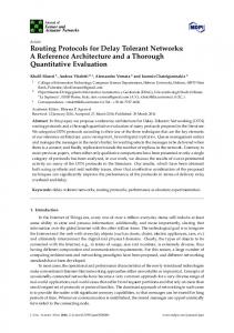
In this chapter, we compare the performance of RBAR with other schemes under different delay requirements. 1) Under long delay requirement: When the delay requirement is long, we hope our scheme RBAR can save energy as long as it satisfies the delay requirement. Figure 4 exhibits the performance of different schemes when the delay requirement is 8000s for all packets, in which Figure 4(a) plots the CDF of delay distributions of different schemes, while Figure 4(b) shows the delivery ratio for packets satisfying delay requirement and the corresponding average energy consumption for each scheme (energy consumption is represented using the number of transmissions to deliver a packet). From Figure 4(a), we can see that Epidemic is the most aggressive scheme. Epidemic can deliver more than 90% of packets with delay less than 2700s and all packets with delay less than 5000s. On the contrary, Direct transmission is the most conservative one, which only delivers 40% of packets with delay less than 2700s and just deliver 80% of all packets within delay requirement finally. As a compromise, Spray and wait predetermines the total number of copies, N, can be replicated, and their performance falls into the range between Epidemic and Direct transmission. The larger N is, the closer it approaches to Epidemic. However, all the delay distributions of the schemes discussed above follow a certain trend, while RBAR is dynamically adjusted along the time. As we observe,

1

CDF of delay distribution

0.8 0.7 0.6 0.5 Epidemic Spray and wait (N=7) Spray and wait (N=5) Spray and wait (N=3) Spray and wait (N=2) RBAR (upper) RBAR RBAR (lower) Direct transmission

0.4 0.3 0.2 0.1 0

0

1000

2000

3000

4000

5000

6000

7000

8000

Time

6 0.8 5

0.7 0.6

4

0.5 3

0.4 0.3

2

0.2 1 0.1 0

EP

DT

RBAR

SW2

SW3

SW5

SW7

SW8

0

Schemes

(a) CDF of delay distribution. Fig. 4.

7

0.9

Number of transmissions

Delivery ratio in delay requirement

1 0.9

(b) Delivery ratio and energy consumption.

Comparison of different schemes under long delay requirement.

RBAR is the same as Direct transmission before the delay around 4000s, this is because RBAR is in the first phase of source forwarding to save energy during this period. After that, the source has to replicate copies to guarantee the packet can be delivered within the delay requirement, resulting the rapidly increased CDF and satisfied final delivery ratio. This means that RBAR is well controlled during the replication procedure and adaptively adjusted according to the delay requirement. Moreover, we also plot the upper and lower bounds for RBAR according to equations 13 and 14 respectively, and demonstrate that the simulation result confirms our analysis. As an evidence from another perspective, Figure 4(b) plots the delivery ratio in delay requirement and energy required in different schemes. Clearly we can see that Epidemic achieves the highest delivery ratio and consumes the most energy, while Direct transmission is on the opposite side with lowest delivery ratio and lowest energy consumption. Similarly, Spray and wait still falls between Epidemic and Direct transmission, in which the larger number of N means more replications and more energy consumption with higher delivery ratio. RBAR also shows good performance with satisfied delays and reasonably low energy consumption compared with others. 2) Under short delay requirement: To demonstrate that RBAR can be adaptively adjusted, we now compare the performance under short delay requirement of 4000s in Figure 5. Correspondingly, when the delay requirement is short, RBAR should perform aggressively at the beginning to satisfy the delay requirement. In Figure 5(a), Epidemic, Direct transmission and Spray and wait all exhibit very similar trends as their counterparts in Figure 4. However, RBAR is totally different, which replicates packets aggressively approaching Epidemic at the very beginning. The reason behind this phenomenon is that, under very short delay requirement, RBAR can directly enter the second phase of copy replication to speed up the replication procedure. Comparing Figures 4(b) and 5(b), we can clearly observe the benefits of RBAR over other schemes. Epidemic is always too aggressive and Direct transmission is always too conservative. For Spray and wait with N = 2, although it achieves low energy consumption under long delay requirement, it leads to very low delivery ratio under short delay requirement. While for Spray and wait with N = 7, it achieves satisfied delivery ratio

under short delay requirement, but also causes huge energy consumption under long delay requirement. Comprehensively, RBAR dynamically adjusts the redundancy and always uses reasonably low energy to satisfy different delay requirements. 3) RBAR is adaptive: As we have discussed, traditional DTN routing schemes do not differentiate packets with various delay requirements, while RBAR adaptively changes the replication strategy to satisfy the requirements. Figures 6(a) and (b) closely examine the difference by plotting the delivery ratio and average number of transmissions for different schemes when the delay requirement increases. For Epidemic, Direct transmission and Spray and wait, they always follow one single replication principle and do not consider the delay requirement, thus the average number of transmissions is almost constant but the percentage of packets delivered with requirements changes significantly. On the contrary, RBAR can always achieve constant delivery ratio with reasonably low energy in accordance to the specific delay requirements. 4) Under hybrid delay requirement: As we observe from Figure 6, under a certain delay requirement, some schemes can get similar delivery ratio as RBAR, while some other schemes may achieve similar energy consumption as RBAR. However, none of them can fulfill these performance metric simultaneously. In this simulation, we examine the performance under hybrid delay requirements. We assume a packet is assigned a emergency level p when it is generated according to the content, which ranges from 0 to 100 with uniform distribution and the delay requirement is determined as D(p) = ap + b, where a = 50 and b = 4000. We compare the performance of different schemes in Figure 7. In Figure 7(a), we observe that RBAR is different from others with various trends of CDF of delay distribution at different time, because RBAR adjusts the redundancy and put different efforts at different time. So RBAR achieves the best tradeoff between delivery ratio and energy consumption as shown in Figure 7(b). 5) When battery is constrained: Lastly we explore the performance when the precious battery resource is constrained. Since underwater sensor nodes are powered by battery, which is hard, if not impossible, to be replaced. A wise scheme in UWSN should always be energy friendly. Figure 8 compares different schemes by setting the battery for each node to support 1200 transmissions. Obviously, with constrained

Delivery ratio in delay requirement

1

CDF of delay distribution

0.8 0.7 0.6 0.5 0.4 RBAR Epidemic Spray and wait (N=2) Spray and wait (N=3) Spray and wait (N=5) Spray and wait (N=7) Direct transmission

0.3 0.2 0.1 0

0

500

1000

1500

2000

2500

3000

3500

5

0.8 0.7

4

0.6 0.5

3

0.4 2

0.3 0.2

1

0.1 0

4000

6

0.9

EP

DT

RBAR

Time

SW2

SW3

SW5

SW7

SW8

Schemes

(a) CDF of delay distribution. Fig. 5.

Number of transmissions

1 0.9

(b) Delivery ratio and energy consumption.

Comparison of different schemes under short delay requirement. 5.5 Epidemic Spray and wait (N=7) Spray and wait (N=5) RBAR (simulation) RBAR (analysis) Spray and wait (N=3) Spray and wait (N=2) Direct transmission

Average number of transmissions

1 0.95

0.8 0.75 RBAR (analysis) Epidemic Spray and wait (N=7) RBAR (simulation) Spray and wait (N=5) Spray and wait (N=3) Spray and wait (N=2) Direct transmission

0.7 0.65 0.6 0.55 4000

5000

6000

7000

4 3.5 3 2.5 2 1.5 1 0.5 0 4000

5000

Delay requirement

(a) Delivery ratio under different delay requirements.

1

1 0.9

0.8

0.8

0.7 0.6 0.5 0.4 Epidemic Spray and wait (N=7) Spray and wait (N=5) RBAR Spray and wait (N=2) Direct transmissions

0.2 0.1 0

0

1000

2000

3000

4000

5000

6000

7000

8000

6

5

0.7

4

0.6 0.5

3

0.4 2

0.3 0.2

1

0.1

9000

Time

(a) CDF of delay distribution. Fig. 7.

8000

Performance of schemes under different delay requirements.

0.9

0.3

7000

(b) Average number of transmissions under different delay requirements.

Average Delivery ratio

CDF of delay distribution

Fig. 6.

6000

Delay requirement

8000

Number of transmissions

Delivery ratio

0.9 0.85

5 4.5

0

EP

DT

RBAR

SW2

SW5

SW7

0

Schemes

(b) Delivery ratio and energy consumption.

Comparison of different schemes under hybrid delay requirement.

battery resource, Epidemic can no longer achieve the highest delivery ratio, because it is too aggressive to replicate copies and wastes resource. While RBAR reaches the highest delivery ratio and reasonably low energy consumption, which relies on the adaptive resource allocation based on the different delay requirements. In this special case, Spray and wait with N = 3 performs similarly. However, for other cases, it may not be a good candidate but RBAR can always fit into different situations.

VI. C ONCLUSION In this paper, we present redundancy based adaptive routing (RBAR) for underwater DTNs. RBAR is dedicated for networks where all nodes and inter-contact time are independent and identically distributed. In these networks, utility based routing schemes are challenging since it is hard to determine which relay is better than others, so RBAR is a good alternative by utilizing redundancy to increase the probability of delivery. Meanwhile, it provides corresponding qualities for various packets with different delay requirements. RBAR explicitly controls the replication procedure and the

0.8

0.8

0.7 0.6 0.5 0.4 Spray and wait (N=3) RBAR Spray and wait (N=2) Spray and wait (N=5) Direct transmissions Spray and wait (N=7) Epidemic

0.3 0.2 0.1 0

0

1000

2000

3000

4000

5000

6000

7000

8000

4

0.7 0.6

3

0.5 0.4

2

0.3 0.2

1

0.1

9000

Time

(a) CDF of delay distribution. Fig. 8.

5

Number of transmissions

1 0.9

Average delivery ratio

CDF of delay distribution

1 0.9

0

EP

DT

RBAR

SW2

SW3

SW5

SW7

Schemes

(b) Delivery ratio and energy consumption.

Comparison of different schemes under hybrid delay requirement and battery constraint.

number of copies in the network all the time, so it guarantees the in-time delivery and better resource reallocation than others. Through extensive simulations, we demonstrate that RBAR can provide delivery diversity to applications with different delay requirements and achieve a good trade-off among delivery ratio, delay and energy consumption. R EFERENCES [1] J.-H. Cui, J. Kong, M. Gerla, and S. Zhou, “Challenges: Building Scalable Mobile Underwater Wireless Sensor Networks for Aquatic Applications,” IEEE Network, Special Issue on Wireless Sensor Networking, vol. 20, no. 3, pp. 12–18, 2006. [2] S. Jain, K. Fall, and R. Patra, “Routing in a Delay Tolerant Network,” in Proc. of SIGCOMM, Portland, Oregon, USA, September 2004. [3] A. Vahdat and D. Becker, “Epidemic Routing for Partially Connected Ad Hoc Networks,” tech. rep. Duke University, April 2000. [4] T. Spyropoulos, K. Psounis, and C. S. Raghavendra, “Spray and Wait: an Efficient Routing Scheme for Intermittently Connected Mobile Networks,” in Proc. of SIGCOMM, Philadelphia, Pennsylvania, USA, 2005. [5] A. Lindgren, A. Doria, and O. Schel´en, “Probabilistic routing in intermittently connected networks,” SIGMOBILE Mob. Comput. Commun. Rev., vol. 7, no. 3, 2003. [6] K. A. Harras, K. C. Almeroth, and E. M. Belding-Royer, “Delay Tolerant Mobile Networks (DTMNs): Controlled Flooding in Sparse Mobile Networks,” Lecture Notes in Computer Science, May 2005. [7] J. Xue, X. Fan, Y. Cao, J. Fang, and J. Li, “Spray and Wait Routing Based on Average Delivery Probability in Delay Tolerant Network,” Networks Security, Wireless Communications and Trusted Computing, International Conference on, vol. 2, 2009. [8] W. Gao, Q. Li, B. Zhao, and G. Cao, “Multicasting in Delay Tolerant Networks: a Social Network Perspective,” in Proceedings of the tenth ACM international symposium on Mobile ad hoc networking and computing, pp. 299–308, ACM, 2009. [9] C. Lee, D. Chang, Y. Shim, N. Choi, T. Kwon, and Y. Choi, “Regional Token Based Routing for DTNs,” in Proc. of ICOIN, Chiang Mai, Thailand, JAN 2009. [10] Q. Yuan, I. Cardei, and J. Wu, “Predict and Relay: an Efficient Routing in Disruption-tolerant Networks,” in Proc. of ACM MOBIHOC, New Orleans, LA, USA, 2009. [11] J. Burgess, B. Gallagher, D. Jensen, and B. N. Levine, “MaxProp: Routing for Vehicle-Based Disruption-Tolerant Networks,” in Proceedings of 25th IEEE International Conference on Computer Communications, 2006. [12] A. Balasubramanian, B. N. Levine, and A. Venkataramani, “DTN Routing as a Resource Allocation Problem,” tech. rep., University of Massachusetts Amherst, Amherst, MA. [13] E. P. Jones, L. Li, and P. A. Ward, “Practical Routing in Delay-tolerant Networks,” in Proc. of WDTN, Philadelphia, PA, USA, September 2005. [14] J. Wu, M. Lu, and F. Li, “Utility-Based Opportunistic Routing in MultiHop Wireless Networks,” in Proc. of IEEE ICDCS, Washington, DC, USA, 2008. [15] I. Cardei, C. Liu, J. Wu, and Q. Yuan, “DTN Routing with Probabilistic Trajectory Prediction,” in Proc. of WASA, Dallas, Texas, USA, 2008.

[16] C. Liu and J. Wu, “An Optimal Probabilistic Forwarding Protocol Delay Tolerant Networks,” in Proc. of ACM MOBIHOC, New Orleans, LA, USA, 2009. [17] R. Groenevelt, P. Nain, and G. Koole, “Message Delay in MANET,” SIGMETRICS Perform. Eval. Rev., vol. 33, no. 1, pp. 412–413, 2005. [18] T. Spyropoulos, K. Psounis, and C. S. Raghavendra, “Spray and Wait: an Efficient Routing Scheme for Intermittently Connected Mobile Networks,” in Proceedings of the 2005 ACM SIGCOMM workshop on Delaytolerant networking, pp. 252–259, ACM, 2005. [19] S. M. Ross, Introduction to Probability Models. Elsevier Science & Technology Books, 9th ed., November 2006.