Efficient Routing in Delay Tolerant Networks with ... - CiteSeerX

Proc. 7th IEEE International Conference on Mobile Ad-hoc and Sensor Systems,IEEE MASS 2010, San Francisco, CA, November 8-12, 2010

Efficient Routing in Delay Tolerant Networks with Correlated Node Mobility Eyuphan Bulut, Sahin Cem Geyik, Boleslaw K. Szymanski Department of Computer Science and Center for Pervasive Computing and Networking Rensselaer Polytechnic Institute, 110 8th Street, Troy, NY 12180, USA {bulute, geyiks, szymansk}@cs.rpi.edu Abstract—In a delay tolerant network (DTN), nodes are connected intermittently and the future node connections are mostly unknown. Since in these networks, a fully connected path from source to destination is unlikely to exist, message delivery relies on opportunistic routing. However, effective forwarding based on a limited knowledge of contact behavior of nodes is challenging. Most of the previous studies looked at only the pairwise node relations to decide routing. In contrast, in this paper, we analyze the correlation between the meetings of each node with other nodes and focus on the utilization of this correlation for efficient routing of messages. We introduce a new metric called conditional intermeeting time, which computes the average intermeeting time between two nodes relative to a meeting with a third node using only the local knowledge of the past contacts. Then, we show how we can utilize the proposed metric on the existing DTN routing protocols to improve their performance. For shortest-path based routing protocols in DTNs, we propose to route messages over conditional shortest paths in which the link cost between nodes are defined by conditional intermeeting times. Moreover, for metric-based forwarding protocols, we propose to use conditional intermeeting time as an additional delivery metric while making forwarding decisions of messages. Our trace-driven simulations on three different datasets show that the modified algorithms perform better than the original ones.

I. I NTRODUCTION Delay tolerant networks (DTN) [1]-[3], also called as intermittently connected mobile networks (ICMN), are wireless networks in which at any given time instance, the probability that there is an end-to-end path from a source to a destination is low. This is caused by the high mobility and low density of the nodes in the network. This property makes the routing of messages in DTNs a challenging problem. The conventional solutions do not generally work in DTNs because they assume that the network is stable most of the time and failures of links between nodes are infrequent. Therefore, the routing problem is still an active research area in DTNs [4]. With the advent of DTNs, store-carry-and-forward paradigm has been widely applied to routing. When a node This research was sponsored by US Army Research Laboratory and the UK Ministry of Defence and was accomplished under Agreement Number W911NF-06-3-0001 and under Cooperative Agreement Number W911NF-092-0053. The views and conclusions contained in this document are those of the authors, and should not be interpreted as representing the official policies, either expressed or implied, of the US Army Research Laboratory, the U.S. Government, the UK Ministry of Defense, or the UK Government. The US and UK Governments are authorized to reproduce and distribute reprints for Government purposes notwithstanding any copyright notation hereon.

has a message but no connection to any other node in the network, it stores the message in its buffer and carries the message until it meets a new node that does not have this message. If the encountered node is assessed to be useful in the delivery of the message, then the message is transferred to it. Several DTN routing algorithms based on this paradigm have been proposed recently. In each, different techniques (single-copy [5], multi-copy [6]-[8], erasure coding [9] [10]) with slightly different goals have been utilized. A survey of previous DTN routing algorithms can be found in [11]. Since DTNs consist of mobile agents that contact intermittently, recent studies on DTN routing have focused on the analysis of real mobility traces (human [16] [17], vehicular [18] etc.) and utilized extracted characteristics of the mobile objects on the design of forwarding algorithms for DTNs. These designs proposed in previous work led us to the following conclusions: ∙

∙

∙

The pairwise intermeeting times between the nodes usually follow a log-normal distribution [19] [20] so that they are not memoryless1 . This makes future contacts of nodes dependent on their past. Most of the previous routing protocols that make the forwarding decisions at node meetings use a metric (encounter frequency [15], time elapsed since last encounter [21] [22], social similarity [23]-[25] etc.) computed from the pairwise relations of nodes with the destination node only. They do not use the information of ‘meeting with each other’ while computing their delivery metrics. The mobility of many real objects are non-deterministic but periodic [27]. For example, in a cyclic MobiSpace [27], if two nodes were frequently in contact at a particular time in previous cycles, then they are likely to meet around the same time in the next cycle.

The above three key observations motivated us to do the research presented in this paper that utilizes the correlation between the meetings of nodes for designing more efficient routing algorithms. Hence, we introduce a new link metric, conditional intermeeting time, that computes the average intermeeting time between two nodes relative to a meeting 1 Assume that 𝑋 is the random variable representing the intermeeting time between two nodes, then the meetings are memoryless if 𝑃 (𝑋 > 𝑠+𝑡 ∣ 𝑋 > 𝑡) = 𝑃 (𝑋 > 𝑠) for 𝑠, 𝑡 > 0 holds.

with a third node using only the local knowledge of the past contacts. For example, with 𝜏𝐴 (𝐷, 𝐵), we define the conditional intermeeting time of node 𝐴 with destination 𝐷 given the condition that it has just 𝐵 as the average time it took in the past (computed from previous contact history) to meet with 𝐷 after its meeting with 𝐵. Hence, at each meeting of node 𝐴 with a potential destination node 𝐷, we compute the meeting frequency of 𝐴 with 𝐷 conditional on meetings with all the other nodes node 𝐴 met since its last meeting with node 𝐷. In the paper, we discuss how this metric addresses all the above mentioned three key observations. Moreover, note that this definition of intermeeting times is also meaningful in terms of the context of routing of messages because the messages are received from a node and given to another node on the way towards the destination. Moreover, the conditional intermeeting time represents the duration that a node holds the message throughout routing. We provide the analysis of conditional intermeeting time and discuss when and why it can be beneficial for providing better information to nodes within the context of routing. We also present statistical results from three different data sets (RollerNet [20], Cambridge [30], Haggle [32]) which contain the contact traces of real objects logged during real life experiments. To show the benefit of this metric, we propose improvements on existing DTN routing protocols. Firstly, for the algorithms which route messages over shortest paths (SP) [12] [14], we propose to use conditional intermeeting times rather than standard intermeeting times and route the messages over conditional shortest paths (CSP). Secondly, for the algorithms which make message forwarding decisions depending on a delivery metric (we call them metric-based forwarding algorithms), we propose to use conditional intermeeting time as a secondary delivery metric and allow the forwarding of messages if and only if both the algorithm’s original delivery metric and conditional intermeeting time suggest to forward the message to the encountered node. Through real-trace-driven simulations on three data sets, we compare the modified protocols with the original ones. The results show that modifications improve performances of those protocols. This shows that the conditional intermeeting time represents inter-node link costs well (in the context of routing) guiding forwarding decisions effectively while routing a message. In short, the contributions of this paper are four-fold: 1) A new metric, conditional intermeeting time is proposed; it computes the average intermeeting time between two nodes relative to a meeting with a third node using only the local knowledge of the past contacts. 2) The analysis of the proposed metric is presented to show significance of the metric for routing. 3) Modification of the existing DTN routing protocols by using conditional intermeeting time metric is discussed. 4) Real-trace-driven simulations are performed and the performance improvement achieved in the updated versions of the existing algorithms on three different data sets

are shown. Thus, the benefit of conditional intermeeting time in making effective decisions in DTN routing is shown experimentally. The remaining of the paper is organized as follows. In Section II, we describe the proposed metric in detail and explain how a node can compute it from its previous contacts. In Section III, we give the analysis of proposed metric. In Section IV, we describe how the conditional intermeeting time can be used to modify existing DTN routing algorithms for performance improvement. In Section V, we present the details of real-trace-driven simulations in which we compare the performance of modified algorithms with the performances of original algorithms. Finally, we offer conclusion and outline the future work in Section VI. II. C ONDITIONAL I NTERMEETING T IME Recently, the research community working on routing algorithms in DTNs has focused on the analysis of real mobility traces to understand the main characteristics of mobile objects. Many experiments in different environments (office [19], conference [32], city [30], skating tour [20]) with different objects (human [16], bus [18], zebra [31]) and with variable number of attendants were performed. From the analysis of the data sets collected during these experiments, significant results about the aggregate and pairwise mobility characteristics of real objects were obtained. As opposed to the random mobility models [26] according to which the intermeeting time between pairs follow an exponential distribution, recent analysis [19] [20] on real mobility traces showed that the intermeeting times between most (more than 99% in many datasets) of the node pairs fit to log-normal distribution. However, this revokes the validity of a common assumption [8] [13] [22] that the pairwise intermeeting times are exponentially distributed and memoryless, and it makes the pairwise contacts between nodes dependent on their pasts. As a first consequence of this, the residual time until the next meeting of two nodes can be predicted more accurately depending on the condition that they have not met during the last 𝑡 time units [19]. However, the dependence of future contacts on the past of nodes can provide more than this. The nodes can also benefit from their past contacts to predict their future contacts more accurately. Previous work have used pairwise node relations in the design of DTN routing protocols while making effective forwarding decisions. The more frequently a node meets with destination, the higher probability it can deliver a message to the destination. Therefore, in the meeting of two nodes, keeping the message in the node with smaller average intermeeting time with destination increases the delivery probability. However, an important aspect here is that nodes receive messages from a node and forward it to another node. That is, the duration that a node holds a message is between its contacts with two different nodes. Depending on the above facts, we propose a new metric called conditional intermeeting time to define the node relations more precisely within the context of routing. This metric

5 units

B

2 units

4 time units/cycle

3 time units/ cycle

A 0

C

5

11 14 16 6 units

A

2 time units cycle

CB

B

2 units

CB

B

23 25

30

7 units

C

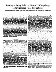
Fig. 1: A physical cyclic MobiSpace with a common motion cycle of 12 time units.

computes the average intermeeting time between two nodes relative to a meeting with a third node using only the local knowledge of the past contacts2 . The proposed metric can also provide more accuracy if the nodes move in a cyclic MobiSpace [27]. According to the definition of cyclic MobiSpace, if two nodes contact frequently at a particular time in previous cycles, the probability that they will be in contact around the same time in the next cycle is high. In Figure 1, a sample cyclic MobiSpace with three objects is illustrated. The common motion cycle is 12 time units. In this example, the discrete probabilistic contacts between 𝐴 and 𝐵 happen in every 12 time units (1, 13, 25..) and the discrete probabilistic contacts between 𝐵 and 𝐶 occur in every 6 time units (2, 8, 14..). When we consider intermeeting time between nodes 𝐵 and 𝐶, we can expect that node 𝐵 will forward its message to node 𝐶 in 6 time units, however conditional intermeeting time of 𝐵 with 𝐶 based on the condition that it has met (received the message from) node 𝐴 lets us know that the message will be forwarded to node 𝐶 within 1 time unit. In a DTN, each node can keep and update the list of its contacts and the previous meeting times with each of them during its lifetime. Then, utilizing this information, each node can find the values of both of their standard and conditional intermeeting times with their neighbors. Let 𝜏𝐴 (𝐵∣𝐶) denote the conditional intermeeting time of node 𝐴 with node 𝐵 given that it has met node 𝐶. It represents the average time that elapses from the time 𝐴 has met 𝐶 to the time it first meets 𝐵. Hence, the standard intermeeting time between 𝐴 and 𝐵 can be denoted as 𝜏𝐴 (𝐵∣𝐵) (or shortly 𝜏𝐴 (𝐵)). To find the conditional intermeeting time of 𝜏𝐴 (𝐵∣𝐶), each time node 𝐴 meets node 𝐶, it starts a different timer. When it meets node 𝐵, it takes the sum of the values on these timers and also notes the number of timers it has started before deleting them. This computation is repeated again each time node 𝐶 is encountered. Then, dividing the sum of time values 2 Note that, the proposed metric is different than conditional residual time (CRT) proposed by Srinivasa et al. in [19]. While CRT computes the remaining time for the meetings of two nodes based on the condition that the nodes have not met each other for some time, our metric computes the residual time to the next meeting of two nodes based on the condition that one of the nodes met with a third node. As we will see in analysis section, CRT is a special case of conditional intermeeting time in which the distribution of passed time since the last meeting is not considered.

C 34

time

4 units 9 units

Fig. 2: Example meeting times of node 𝐴 with nodes 𝐵 and 𝐶. While the values in the upper part are used in the computation of 𝜏𝐴 (𝐵∣𝐶), the values in the lower part are used in the computation of 𝜏𝐴 (𝐶∣𝐵). collected from each timer by the total count of all timers used gives the value of 𝜏𝐴 (𝐵∣𝐶). We can also use a sliding window with an appropriate size over the past contacts [14] to make the conditional intermeeting value more local and current. Consider Figure 2 which shows the sample contact times of a node 𝐴 with its neighbors 𝐵 and 𝐶. Node 𝐴 meets with node 𝐵 at times {5, 16, 25, 30} and with node 𝐶 at times {11, 14, 23, 34}. Then, following the procedure described above, 𝜏𝐴 (𝐵∣𝐶) = 3 and 𝜏𝐴 (𝐶∣𝐵) = 6.5 units. III. A NALYSIS In this section, we give the analysis of conditional intermeeting time and show why it is significant in accurate prediction of future meetings within the context of routing. Assume that node 𝐴 has two different contacts, 𝐵 and 𝐶, and the sets 𝑆𝐵 and 𝑆𝐶 include the meeting times of node 𝐴 with nodes 𝐵 and 𝐶 in order during the time frame [0, 𝑇 ], respectively. 𝑆𝐵 = {𝐵1 , 𝐵2 , 𝐵3 , . . . 𝐵𝑛 }, n meetings 𝑆𝐶 = {𝐶1 , 𝐶2 , 𝐶3 , . . . 𝐶𝑚 }, m meetings Furthermore, assume that the intermeeting time of node 𝐴 with node 𝐵 is well represented by a random variable 𝑋1 while the intermeeting time of node 𝐴 with 𝐶 is well represented by a random variable 𝑋2 with the CDF 𝐷2 (𝑥) and probability density 𝑑2 (𝑥) = 𝐷2′ (𝑥). To find 𝜏𝐴 (𝐶∣𝐵), we need to compute the following (without loss of generality, we assume that 𝐶𝑚 ≥ 𝐵𝑛 ): ∑𝑚 𝑘=1 (𝐶𝑑(𝑘) − 𝐵𝑘 ) , 𝜏𝐴 (𝐶∣𝐵) = 𝑚 where, 𝑑(𝑘) = min{𝑖 : 𝐶𝑖 ≥ 𝐵𝑘 }. The conditional intermeeting time of node 𝐴 with node 𝐶 under the condition that it has met node 𝐵 is then a random variable that we will denote as 𝑌 . Then 𝜏𝐴 (𝐶∣𝐵) = 𝐸[𝑌 ]. Let’s consider 𝑗 𝑡ℎ meeting of node 𝐴 with node 𝐵 and denote 𝑡 = 𝐵𝑗 − 𝐶𝑑(𝑗)−1 . Consider a family of random variables 𝑌 (𝑡)’s with CDFs 𝐷𝑡 (𝑥) and probability densities 𝑑𝑡 (𝑥), then: 𝐷𝑡 (𝑦)

=

𝑑𝑡 (𝑦)

=

𝐷2 (𝑦 + 𝑡) − 𝐷2 (𝑡) 1 − 𝐷2 (𝑡) 𝑑2 (𝑦 + 𝑡) 1 − 𝐷2 (𝑡)

Haggle Traces

RollerNet Traces

Cambridge Traces

12 10 8 6 4 2 0 40 40 20

1000

500

0 60 60

40

20 0

C

0

3

2

1

0 30

0

0

20

10

10 0

C

B

C−Map of node 33 in RollerNet traces

40

30

20

20

C

C−Map of node 21 in Haggle traces

x 10

40

20

B

Conditional Intermeeting time (sec)

5

Conditional Intermeeting time (sec)

Conditional Intermeeting time (sec)

4

x 10

0

B

C−Map of node 2 in Cambridge traces 35

60

35

30

50 30

25 40

25

C

C

C

20 20

30

15 15 20

10

10 10

5 0

0

10

20 B

30

0

40

(a) C-Map of node 21 in Haggle traces

5

0

10

20

30 B

40

50

60

0

0

5

10

15

20

25

30

35

B

(b) C-Map of node 33 in RollerNet traces

(c) C-Map of node 2 in Cambridge traces

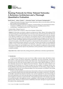
Fig. 3: C-Maps of popular nodes in three datasets. In figures, 𝐵 represents the id of the node already met and 𝐶 represents the id of the node to be met. ∫∞ 𝐸[𝑌 (𝑡)]

= =

𝑦=0

𝑦𝑑2 (𝑦 + 𝑡)𝑑𝑦

1 − 𝐷2 (𝑡) ∫∞ (1 − 𝐷2 (𝑦))𝑑𝑦 𝑦=𝑡

1 − 𝐷2 (𝑡) When 𝑋1 and 𝑋2 are exponentially distributed random variables, then 𝐷𝑡 (𝑥) = 𝐷2 (𝑥), showing the memoryless property of exponential distribution. However, as the previous work suggests, 𝑋1 and 𝑋2 fit well with log-normal distribution. Then: ( )] 2 [ 𝜎2 ln 𝑡−(𝜇2 +𝜎22 ) √ 𝑒𝜇2 + 2 1 − erf 𝜎2 2 ] [ 𝐸[𝑌 (𝑡)] = −𝑡 ln 𝑡−𝜇 √ 1 − erf 𝜎 22 2

where 𝑒𝑟𝑓 is error function and 𝜇2 and 𝜎2 are mean and variance of 𝑋2 , respectively. Since in this case, as well in general, the expected value of 𝑌 (𝑡) depends on the value of 𝑡, then, denoting by 𝑑𝐴𝐶𝐵 (𝑡) the probability density of the time difference between the meeting of node 𝐴 with 𝐶 to time of meeting of node 𝐴 with 𝐵 before 𝐴 meets 𝐶, we get: ∫ ∞ ∫ ∞ (1 − 𝐷 (𝑦))𝑑𝑦 2 𝑦=𝑡 𝑑𝐴𝐶𝐵 (𝑡)𝑑𝑡 𝐸[𝑌 ] = 1 − 𝐷 2 (𝑡) 𝑡=0 Clearly, 𝐸[𝑌 ] depends on probability density function 𝑑𝐴𝐶𝐵 (𝑡) that is defined by the correlation between the meet-

ings of node 𝐴 with nodes 𝐵 and 𝐶. Due to the nature of DTNs, and also the possible cyclic behavior of nodes [27], there is often a repeating pattern between the meetings of node 𝐴 with node 𝐵 and 𝐶, creating a strong correlation. Consequently, 𝐸[𝑌 ] strongly depends on the aforementioned correlation. Given 𝐴, to see the distribution of 𝜏𝐴 (𝐶∣𝐵) according to different 𝐵 and 𝐶 nodes, we computed the average conditional intermeeting time maps (C-Map) of the most popular nodes (having the highest total meeting count with other nodes) in three different datasets. In Figure 3, we show these results. For each dataset, the upper plot shows the 3D view of 𝜏𝐴 (𝐶∣𝐵) and the lower plot shows the contour plot displaying the isolines of 𝜏𝐴 (𝐶∣𝐵). The darker the color in the plots, the smaller the 𝜏𝐴 (𝐶∣𝐵) values. Interestingly, the diagonals and the 𝐴𝑡ℎ row and column in the plots are the darkest places because 𝜏𝐴 (𝐶∣𝐵) values are assumed zero in these cases. Moreover, if there is no instance of the case in which node 𝐴 meets node 𝐶 after it meets node 𝐵, we assumed 𝜏𝐴 (𝐶∣𝐵) = −1. If there were no correlation between the meetings of node A with other nodes, 𝜏𝐴 (𝐶∣𝐵) would have been the same for all 𝐵’s other than 𝐴 or 𝐶 and entire rows would have been of the same color in contour plots. In contrast, we observe different

colors within the rows, demonstrating that the meetings of node 𝐴 with different nodes are not independent of each other. Indeed this result matches with real world scenarios. For example, consider the meetings of a man who goes from home to work every morning. After meeting his family members (while leaving home), he meets later his office friends. Yet, on the way to his office, he meets the security guard at the gate of his workplace a few moments before meeting his office friends. In other words, the meetings of the man with his office friends is correlated with his meetings with security guard. IV. P ROPOSED A LGORITHMS In this section, we present two different utilization of conditional intermeeting time in existing DTN routing algorithms. In the first part, we look into the shortest path based routing algorithms and propose to use conditional shortest paths to route messages. Then, in the second part, we propose to revise message forwarding decision of metric-based forwarding algorithms by including the conditional intermeeting time. A. Shortest Path based Routing 1) Overview: Shortest path routing (SPR) protocols for DTNs are based on the designs of routing protocols for traditional networks. The links between each pair of nodes are assigned a cost and messages are forwarded over the shortest paths between the source and the destination. Furthermore, the dynamic nature of DTNs is also addressed in these designs. Two of the common metrics used to define the link cost are minimum expected delay (MED [14]) and minimum estimated expected delay (MEED [14]). These metrics compute the expected waiting time plus the transmission delay between each pair of nodes. However, while the former uses the future contact schedule, the latter uses only observed contact history. In this paper, we are interested in neither the suitability of SPR algorithms for DTNs nor the scalability and complexity of their designs as the papers introducing the original algorithms include elaborate discussions of these issues. In this paper, we focus on the enhancements of the performance of SPR algorithms achieved by utilizing our metric, conditional intermeeting time, rather than using standard intermeeting time. To this end, in the rest of this section, we show the necessary changes to the current designs of SPR algorithms. 2) Network Model: We model a DTN as a graph 𝐺 = (𝑉 , 𝐸) where the mobile nodes are represented by vertices (𝑉 ) and the possible connections between these nodes are represented by the edges (𝐸 = 𝐸𝑢 ∪ 𝐸𝑏 ), which, unlike previous DTN graph models, allows for multiple and both unidirectional (𝐸𝑢 ) and bidirectional (𝐸𝑏 ) edges between the nodes. The neighbors of a node 𝑖 are denoted by 𝑁 (𝑖) and the edge sets are given as follows: 𝐸𝑏 𝐸𝑢

= =

{(𝑖, 𝑗) ∣ ∀𝑗 ∈ 𝑁 (𝑖)} where, 𝑤(𝑖, 𝑗) = 𝜏𝑖 (𝑗) = 𝜏𝑗 (𝑖) {(𝑖, 𝑗) ∣ ∀𝑗 ∕= 𝑘 ∈ 𝑁 (𝑖)} where, 𝑤(𝑖, 𝑗) = 𝜏𝑖 (𝑗∣𝑘)

Note that there can be multiple unidirectional edges (𝐸𝑢 ) between any two nodes but these edges differ from each other

C TA(C|B)

TA(B)

TA(C)

TA(C|D) TA(D)

A

TA(D|C)

TA(B|C) TA(B|D)

B

TA(D|B)

D

Fig. 4: A sample DTN graph with four nodes and nine edges. in terms of their weights (𝑤(𝑖, 𝑗)) and the corresponding third node which is the reference point used while computing the conditional intermeeting time. In Figure 4, we illustrate a sample DTN graph with four nodes and nine edges. There are three bidirectional edges with weights of standard intermeeting times and six unidirectional edges with weights of conditional intermeeting times. 3) Conditional Shortest Path Routing: Our algorithm basically finds conditional shortest paths (CSP) for each sourcedestination pair and routes the messages over these paths. We define the CSP from a node 𝑛0 to a node 𝑛𝑑 as follows: 𝐶𝑆𝑃 (𝑛0 , 𝑛𝑑 )

=

{𝑛0 , 𝑛1 , . . . , 𝑛𝑑−1 , 𝑛𝑑 ∣ ℜ𝑛0 (𝑛1 ∣𝑡) + 𝑑−1 ∑ 𝜏𝑛𝑖 (𝑛𝑖+1 ∣𝑛𝑖−1 ) is minimized.} 𝑖=1

Here, 𝑡 represents the time that has passed since the last meeting of 𝑛0 with 𝑛1 and ℜ𝑛0 (𝑛1 ∣𝑡) is the expected residual time to the next meeting of 𝑛0 and 𝑛1 given that they have not met in the last 𝑡 time units. ℜ𝑛0 (𝑛1 ∣𝑡) can be computed as in [19] with parameters of distribution representing the intermeeting time between 𝑛0 and 𝑛1 . It can also be computed in a discrete manner from the observed intermeeting times of 𝑛0 and 𝑛1 . Assume that 𝑛0 observed 𝑘 intermeeting times with 𝑛1 in the past. Let 𝜏𝑛10 (𝑛1 ), 𝜏𝑛20 (𝑛1 ),. . .𝜏𝑛𝑘0 (𝑛1 ) denote these values. Then, discrete computation of ℜ𝑛0 (𝑛1 ∣𝑡) can be defined formally as follows: ∑𝑘 𝑠 𝑠=1 𝑓𝑛0 (𝑛1 ) where, ℜ𝑛0 (𝑛1 ∣𝑡) = ∣{𝜏𝑛𝑠0 (𝑛1 ) ≥ 𝑡 }∣ { 𝑠 𝜏𝑛0 (𝑛1 ) − 𝑡 if 𝜏𝑛𝑠0 (𝑛1 ) ≥ 𝑡 𝑓𝑛𝑠0 (𝑛1 ) = 0 otherwise If none of the 𝑘 observed intermeeting times is bigger than 𝑡 (this case occurs less likely as the the contact history grows), ℜ𝑛0 (𝑛1 ∣𝑡) becomes 0, which is a good approximation. Next, we give an example to show the benefit of CSP over SP. Consider the DTN shown in Figure 5. The weights of edges (𝐴, 𝐶) and (𝐴, 𝐵) show the expected residual time of node 𝐴 with nodes 𝐶 and 𝐵, respectively, in both graphs. The weights of edges (𝐶, 𝐷) and (𝐵, 𝐷) are different in both graphs. While in the left graph, they show the average intermeeting times of nodes 𝐶 and 𝐵 with 𝐷 respectively, in the right graph, they show the average conditional intermeeting times of the same

C R (C|t) =20 A

C 30= TC (D)

A

D

R (B|t) =25 A

B

15= TB (D)

R (C|t) =20 A

A R (B|t) =25 A

Path 1

D B

nodes with 𝐷 relative to their meeting with node 𝐴. From the left graph, we conclude that SP(𝐴, 𝐷) is (𝐴, 𝐵, 𝐷). Thus, it is expected that on average a message from node 𝐴 will be delivered to node 𝐷 in 40 time units. However this may not be the actual shortest delay path. As the weight of edge (𝐶, 𝐷) states in the right graph, node 𝐶 can have a smaller conditional intermeeting time (than the standard intermeeting time) with node 𝐷 assuming that it has met node 𝐴. In other words, node 𝐶 understands its faster transfer capability of messages (received from node 𝐴) to node 𝐷. Hence, in the right graph, CSP(𝐴, 𝐷) is (𝐴, 𝐶, 𝐷) with the path cost of 30 time units. A node-specific view of the network using the aforementioned network model is formed at each node and the standard and conditional intermeeting times of other nodes are collected via epidemic link state protocol as it is described in original study [14]. However, once the weights are known, it is not as easy to find CSPs as it is to find SPs. Consider Figure 6 where the CSP(𝐴, 𝐸) follows path 2 and CSP(𝐴, 𝐷) follows (𝐴, 𝐵, 𝐷). This situation is likely to happen in a DTN, if 𝜏𝐷 (𝐸∣𝐵) ≥ 𝜏𝐷 (𝐸∣𝐶) is satisfied. Running Dijkstra’s or Bellman-Ford algorithm on the current graph structure cannot detect such cases and concludes that CSP(𝐴, 𝐸) is (𝐴, 𝐵, 𝐷, 𝐸). Therefore, to obtain the correct CSPs for each source destination pair, we propose the following transformation on the current graph structure. Given a graph 𝐺 = (𝑉, 𝐸), we obtain a new graph 𝐺′ = (𝑉 ′ , 𝐸 ′ ) where: ⊆ =

𝑉 × 𝑉 and 𝐸 ′ ⊆ 𝑉 ′ × 𝑉 ′ where, {(𝑖𝑗 ) ∣ ∀𝑗 ∈ 𝑁 (𝑖)} and 𝐸 ′ = {(𝑖𝑗 , 𝑘𝑙 ) ∣ 𝑖 = 𝑙} { 𝜏𝑖 (𝑘∣𝑗) if 𝑗 ∕= 𝑘 where, 𝑤′ (𝑖𝑗 , 𝑘𝑙 ) = otherwise 𝜏𝑖 (𝑘)

Remark that the edges in 𝐸𝑏 (in 𝐺) are made directional in 𝐺′ . Also the unidirectional edges (𝐸𝑢 ) between the same pair of nodes in 𝐺 are separated in 𝐸 ′ . This graph transformation keeps all the historical information that conditional intermeeting times require and also keeps only the paths with a valid history. For example, if a path 𝐴, 𝐵, 𝐶, 𝐷 is chosen, then an edge like (𝐶𝐷 , 𝐷𝐴 ) cannot be chosen because of the edge settings in the graph. Hence, only the correct 𝜏 values will be added to the path calculation. To solve the conditional shortest path problem however, we add one vertex for source 𝑆 (apart from its permutations) and one vertex for destination node 𝐷. We also add outgoing edges from 𝑆 to each vertex (𝑖𝑆 ) ∈ 𝑉 ′

D

A

12= TB (D|A)

Fig. 5: An example case where CSP can be different than SP.

𝑉′ 𝑉′

B

10= TC (D|A)

E

C Path 2

Fig. 6: Path 2 may have smaller conditional delay than path 1 even though CSP from 𝐴 to 𝐷 is through 𝐵. with weight ℜ𝑆 (𝑖∣𝑡). Furthermore, for the destination node, 𝐷, we add only incoming edges from each vertex 𝑖𝑗 ∈ 𝑉 ′ with weight 𝜏𝑖 (𝐷∣𝑗) and from 𝑆 with weight ℜ𝑆 (𝐷∣𝑡). In Figure 7, we show a sample transformation of a clique of four nodes to the new graph structure. In the initial graph, all mobile nodes 𝐴 to 𝐷 meet with each other, and we set the source node to 𝐴 and destination node to 𝐷 (we did not show the directional edges in original graph for brevity). Note that we set any path to begin with 𝐴 on transformed graph 𝐺′ , but we also put the permutations of 𝐴, 𝐵 and 𝐶 with each other. Running Dijkstra’s shortest path algorithm on 𝐺′ given the source node 𝑆 and destination node 𝐷 will give shortest conditional path. In 𝐺′ , ∣𝑉 ′ ∣ = 𝑂(∣𝑉 ∣2 ) and ∣𝐸 ′ ∣ = 𝑂(∣𝑉 3 ∣) = ∣𝐸∣3/2 , and therefore Dijkstra’s algorithm will run in 𝑂(∣𝑉 ∣3 ) (with Fibonacci heaps) while computing the original shortest paths (with standard intermeeting times) takes 𝑂(∣𝑉 ∣2 ). Using conditional intermeeting times instead of standard intermeeting times only requires (over original design) extra space to store the conditional intermeeting times and additional processing as complexity of running Dijkstra’s algorithm increases from 𝑂(∣𝑉 ∣2 ) to 𝑂(∣𝑉 ∣3 ). We believe that in current DTNs, wireless devices have enough storage and processing power not to be unduly taxed with such an increase. Moreover, to lessen the burden of collecting and storing link weights, an asynchronous and distributed version of the Bellman-Ford algorithm can be used, as described in [28]. B. Metric-based Forwarding Algorithms 1) Overview: In DTNs, a common routing method is to forward the message to the encountered node that is more likely to meet with destination than the current message carrier. However, making effective forwarding decisions in singlecopy based routing in DTNs is a challenging task. When two nodes meet, one of them forwards a message to the other one if it decides that the message will have a higher chance to be delivered to destination at the other node. In previous work, depending on the observed contact history between nodes, several metrics have been used to define the delivery quality of nodes. Some of the popular ones are encounter frequency [15], time elapsed since last encounter [21] [22], residual time [19] and social similarity [23][25]. For example, in Prophet [15], messages are forwarded to the nodes meeting the destination more frequently.

AB

T (C | B)

A

T (D | B) A

Source

AC

A

BA B

C

A

RA(B|t)

TB(A | C)

TA(D | C)

TB (D | A)

D

T (D | C) B

BC TC(B | A)

D Destination A, B, C and D all meet with each other

T (D | A) C

CA

T (D | B) C

RA(C|t)

CB RA(D|t)

Fig. 7: Graph transformation to solve CSP with 4 nodes where 𝐴 is the source and 𝐷 is the destination.

2) Proposed Revision: According to most of the delivery metrics proposed previously, two encountering nodes make the message forwarding decision depending on their individual relations with the destination node. In some algorithms such as [15] [22], transitivity rule is utilized to reflect the effect of other nodes on the delivery quality of a node but such an approach can be applied to all delivery metrics and it does not reflect the metric’s own feature. To make forwarding decisions of these algorithms more effective, thus to improve their performance, we propose to use conditional intermeeting time as an additional delivery metric. That is, when two nodes meet, they will also compare their conditional intermeeting times with destination and if the current carrier of the message learns that other node has also shorter remaining time (according to conditional intermeeting time) to meet the destination than itself, the message is forwarded. At first glance, this additional condition seems to cut down the number of times the message is forwarded so that the probability of delivery will be reduced. However, as simulation results show, the necessary number of hops are preserved and the less beneficial ones are not performed. Therefore, more effective forwarding decisions are made so that the cost of message delivery declines while the delivery ratio and average delay are maintained (in some cases, even the delivery ratio increases and average delay decreases). V. S IMULATIONS To evaluate the performance of proposed modifications of algorithms, we have built a Java based DTN simulator which uses the traces of real objects. We used traces from three datasets which include the contact times and durations of real objects logged in different DTN environments and we set the network parameters (number of nodes etc.) accordingly. A. Algorithms in Comparison In simulations, we compared existing DTN algorithms with their modifications utilizing conditional intermeeting time in their designs. First, we compared Shortest Path Routing (SPR) with Conditional Shortest Path Routing (CSPR) which is described in Section IV-A3. Then, we compared the existing and

revised versions of two metric-based DTN routing algorithms: Prophet [15] and Fresh [21]. In Prophet, when two nodes, 𝐴 and 𝐵, meet, 𝐴 forwards its message to 𝐵 if and only if its predicted time of delivery to destination 𝐷 is smaller than 𝐵’s predicted time of delivery. In Fresh, 𝐴 forwards the message to 𝐵 only if 𝐵 has a more recent meeting with destination 𝐷 than itself. In the revised versions of these algorithms (we refer to them as C-Prophet and C-Fresh to underline that they use conditional intermeeting time), 𝐴 forwards the message to 𝐵 if 𝜏𝐴 (𝐷∣𝐵) > 𝜏𝐵 (𝐷∣𝐴) is also satisfied (in addition to algorithm’s own forwarding condition). Although we obtained results (showing performance improvement) with many metric-based algorithms (including [19]), we show only the results of two benchmarking algorithms due to lack of space. However, we give the results obtained by Epidemic Routing [6] since it achieves the optimum delivery ratio and delay (at high cost, however). B. Data Sets To evaluate the proposed algorithms, we used traces from the following three data sets. 1) RollerNet Dataset [20]: It includes the opportunistic sightings of Bluetooth devices distributed to 62 rollerbladers in the 3 hour roller tour of Paris in August 20, 2006. 2) Cambridge Dataset [30]: This data includes a number of traces of Bluetooth sightings by 36 students from Cambridge University who were asked to carry the iMotes with them at all times for the duration of the experiment that started on October 28, 2005 and ended on December 21, 2005. 3) Haggle Project Dataset [32]: Among the different experiments performed within Haggle Project, we selected the Bluetooth sightings recorded between the iMotes carried by 41 attendants of Infocom’05 Conference held in Miami. Devices were distributed on March 7th, 2005 between lunch time and 5pm and collected on March 10th, 2005 in the afternoon. C. Performance Metrics We use the following three metrics to compare the algorithms: message delivery ratio, average cost, and routing efficiency. Delivery ratio is the proportion of messages delivered

1

0.8

0.8

0.8

0.6

0.4

SPR CSPR Epidemic

0.2

0

0

10

20 30 Time (min)

40

(a) RollerNet Traces

Message delivery ratio

1

Message delivery ratio

Message delivery ratio

1

0.6

0.4

SPR CSPR Epidemic

0.2

50

0

0

1

2

3 Time (day)

4

(b) Cambridge Traces

5

0.6

0.4

SPR CSPR Epidemic

0.2

6

0

0

0.5

1 Time (day)

1.5

2

(c) Haggle Project Traces

Fig. 8: Comparison of SPR and CSPR: Message delivery ratio vs. time.

to their destinations among all messages generated. Average cost (which is a good indicator of the total power consumption in the network) is the average number of forwardings done per message before delivery. Finally, routing efficiency [33] is defined as the ratio of delivery ratio to the average cost. In the results, we did not give separate plots for delivery delay because they can be obtained from the delivery ratio plots. D. Results To collect several routing statistics, we have generated traffic from the traces of three data sets. For each simulation run, after a warm up period, we generated 5000 messages from a random source node to a random destination node at each 𝑡 seconds. In RollerNet, since the duration of experiment is short, we set 𝑡 = 1s, but for Cambridge and Haggle data sets, we set 𝑡 = 1min and 𝑡 = 30s, respectively. We assume that the nodes have enough buffer space to store every message they receive, the bandwidth is high and the contact durations of nodes are long enough to allow the exchange of all messages between nodes3 . These assumptions are reasonable in view of today’s technology capabilities and are also used commonly in previous studies [29]. Besides, we compare all algorithms in the same conditions. Any change in the current assumptions is expected to affect the performance of compared algorithms in the same way since they use one copy of the message. Moreover, we used a simple MAC model similar to CSMA model. We ran each simulation 10 times with different seeds and in each run we collect statistics by running each algorithm on the same set of messages. All results plotted in figures show the averages of results obtained in all runs (we did not plot the error bars since they were very small). 1) Comparison of CSPR and SPR: Figure 8a shows the delivery ratios achieved in CSPR and SPR algorithms with respect to time (i.e. TTL of messages) in RollerNet traces. Clearly, CSPR algorithm delivers more messages to their destinations than SPR algorithm. Moreover, it achieves lower average delivery delay than SPR algorithm. For example, CSPR delivers 80% of all messages after 17 minutes with 3 We also performed simulations with limited resources (e.g. buffer, bandwidth) and obtained results showing better (but different) performance improvement in revised algorithms over original algorithms. However, we present them in the extended version of the paper due to the lack of space here.

an average delay of almost 6 minutes, while SPR achieves the same delivery ratio only after 41 minutes and with an average delay of 12 minutes. Moreover, although we did not show it here for brevity, average costs in SPR and CSPR are very close (1.48 and 1.52 respectively) to each other (and much smaller than the average cost in epidemic routing which is around 25). We also see the better delivery ratios achieved by CSPR algorithm in Cambridge and Haggle traces in Figure 8b and Figure 8c, respectively. In Cambridge traces, after 6 days, CSPR delivers 78% of all messages with an average delay of 2.6 days, however SPR can only deliver 62% of all messages to their destination with an average delay of 3.2 days. Moreover average costs in SPR and CSPR are 1.73 and 1.78 respectively while it is around 16 in epidemic routing. Similarly, in Haggle traces, with an average cost close to each other, CSPR delivers 87% of all messages by the end of simulation whereas SPR can only achieve 78% delivery ratio. To put this in perspective, compared to Epidemic routing with the highest achievable delivery ratio (94% in Haggle traces with current setting), CSPR lost only 7% of messages, while SPR lost 16% so CSPR achieved more than 55% improvement over SPR. These results show that in the context of routing, conditional intermeeting time provides a better representation of link cost than standard intermeeting time. Therefore, in CSPR, more effective paths with similar average hop counts are selected during the routing of a message towards the destination. Thus, higher delivery ratios with lower end-to-end delays are achieved. In SPR and CSPR algorithms here, we used sourcerouting [12] and let the messages follow the paths which are decided at the source nodes. We also observed similar results in our simulations with other routing approaches (per-hop and per-contact routing [14]). 2) Comparison of revised and original versions of metricbased algorithms: In Figure 9a, we show the delivery ratios achieved in RollerNet traces. Clearly, the modified algorithms provide higher delivery ratio than the original ones. Moreover, as Figure 9b shows, average cost is lower for the modified versus the original algorithms. For example, C-Prophet delivers 90% of all messages after 23 minutes with average delay of 7.8 minutes and average cost of 4.83 hops. However, the original Prophet reaches the same delivery ratio only after 33 minutes with average delay of 13.5 minutes and 17.02 average cost. A

20

15

0.6

0.4 Prophet C−Prophet Fresh C−Fresh Epidemic

0.2

0

0

10

20 30 Time (min)

40

0.4

Prophet C−Prophet Fresh C−Fresh

Prophet C−Prophet Fresh C−Fresh Epidemic

0.35 Routing Efficiency

0.8 Average Cost

Message delivery ratio

1

10

0.3 0.25 0.2 0.15

5

0.1 0.05

0

50

5

(a) Message delivery ratio vs. time

10

15

20

25 30 Time (min)

35

40

45

0

50

0

(b) Average cost vs. time

10

20 30 Time (min)

40

50

(c) Routing Efficiency vs. time

Fig. 9: Comparison of metric-based forwarding algorithms using RollerNet traces 8

0.5 Prophet C−Prophet Fresh C−Fresh

0.8

6

0.6

0.4 Prophet C−Prophet Fresh C−Fresh Epidemic

0.2

0

0

1

2 Time (day)

3

Average Cost

Message delivery ratio

7

Prophet C−Prophet Fresh C−Fresh Epidemic

0.4 Routing Efficiency

1

5 4 3 2

0.3

0.2

0.1

1 0

4

(a) Message delivery ratio vs. time

0.5

1

1.5

2 2.5 Time (day)

3

3.5

4

0

4.5

0

(b) Average cost vs. time

1

2 Time (day)

3

4

(c) Routing Efficiency vs. time

Fig. 10: Comparison of metric-based forwarding algorithms using Cambridge traces 20

15

0.6

0.4 Prophet C−Prophet Fresh C−Fresh Epidemic

0.2

0

0

0.5

1 Time (day)

1.5

(a) Message delivery ratio vs. time

2

0.4 Prophet C−Prophet Fresh C−Fresh

Prophet C−Prophet Fresh C−Fresh Epidemic

0.35 Routing Efficiency

0.8 Average Cost

Message delivery ratio

1

10

5

0.3 0.25 0.2 0.15 0.1 0.05

0

0.5

1 Time (day)

1.5

(b) Average cost vs. time

2

0

0

0.5

1 Time (day)

1.5

2

(c) Routing Efficiency vs. time

Fig. 11: Comparison of metric-based forwarding algorithms using Haggle Project traces

similar situation is also observed between C-Fresh and Fresh. Consequently, routing efficiency is increased more than 100%. When we look at the results obtained from Cambridge and Haggle traces in Figure 10 and Figure 11, we observe a different improvement. As it is seen in Figure 10a and Figure 11a, revised and original versions of algorithms have similar delivery ratios (and therefore similar average delays). However, as Figure 10b and Figure 11b show, average costs in modified versions are lower than they are in original ones. Moreover, in Cambridge traces, the mean hop counts of Prophet, C-Prophet, Fresh and C-Fresh are 5.21, 2.48, 3.83 and 2.53, respectively and in Haggle traces, they are 12.7, 4.98, 5.23 and 3.44. This shows that when conditional intermeeting time is used as an additional delivery metric,

the nodes choose their next hops more effectively so that the cost is decreased while still keeping the original delivery ratio. Therefore, again more than 100% gain is achieved in routing efficiency. From the above results, we see the benefit of conditional intermeeting times in metric-based forwarding algorithms clearly. Moreover, we also observe that in different environments, the improvements obtained thanks to utilization of conditional intermeeting times can be different. In RollerNet traces, we observed improvement in all metrics. However, in Cambridge traces we observed an improvement only in average cost, thus, in routing efficiency. From our initial analysis of the traces, we conclude that this is caused by the repetitive contacts between objects in RollerNet traces. That is, as it is stated in [20], during the tour, fluctuations

in the motion of the rollerbladers cause a typical accordion phenomenon (the topology expands and shrinks with time). When the topology shrinks, nodes are in contact with each other, but when the topology expands, they are disconnected. This property in the contacts of nodes creates a cyclic behavior and lets the proposed algorithms perform better. However, in Cambridge and Haggle traces, the repetitive behavior of node meetings is not clearly detected. From these results, we conclude that the benefit of using conditional intermeeting times in metric based algorithms becomes more pronounced in the environments in which the repetitive motion of nodes is clearly observed. However, even in the environments where this is not the case, average cost of routing can be decreased and routing efficiency can be improved remarkably thanks to use of conditional intermeeting times. VI. C ONCLUSION AND F UTURE W ORK In this paper, we focused on the routing problem in delay tolerant networks (DTN). First, inspired by the results of the recent studies showing that intermeeting times between nodes are not memoryless and the motion patterns of mobile nodes are frequently repetitive, we introduced a new metric called conditional intermeeting time which is the average time that passes from the time a node meets with a neighbor node until the time it meets another one. Next, we presented an analysis of this metric showing why it can be beneficial in proper representation of node relations. Then, we looked at the effects of this metric on existing DTN routing algorithms. To this end, we modified their current designs using conditional intermeeting time. Finally, through real-trace-driven simulations, we evaluated the modified algorithms and demonstrated the superiority of them over original ones. As a future work of our study, we would like to extend the definition of conditional intermeeting time by using more meetings from the contact history. For instance, assume that a node 𝐴 wants to compute its conditional intermeeting time with a node 𝐵 after the time it has met another node 𝐶. Here, we want to differentiate the following two cases which are considered together in our current approach; when node 𝐴 has met node 𝐷 before node 𝐶 and when node 𝐴 has met node 𝐸 before node 𝐶. To apply this algorithm in our work, we plan to use probabilistic context free grammars (PCFG) and utilize the construction algorithm presented in [34]. R EFERENCES [1] P. Juang, H. Oki, Y. Wang, M. Martonosi, L. S. Peh, and D. Rubenstein, Energy-efficient computing for wildlife tracking: design tradeoffs and early experiences with zebranet, in Proceedings of ACM ASPLOS, 2002. [2] Disruption tolerant networking, http://www.darpa.mil/ato/solicit/DTN/. [3] J. Ott and D. Kutscher, A disconnection-tolerant transport for drive-thru internet environments, in Proceedings of IEEE INFOCOM, 2005. [4] Delay tolerant networking research group, http://www.dtnrg.org. [5] J. Burgess, B. Gallagher, D. Jensen, and B. N. Levine, MaxProp: Routing for Vehicle-Based Disruption- Tolerant Networks, in Proc. IEEE Infocom, April 2006. [6] A. Vahdat and D. Becker, Epidemic routing for partially connected ad hoc networks, Duke University, Tech. Rep. CS-200006, 2000. [7] T. Spyropoulos, K. Psounis,C. S. Raghavendra, Efficient routing in intermittently connected mobile networks: The multi-copy case, IEEE/ACM Transactions on Networking, 2008.

[8] E. Bulut, Z. Wang, and B. Szymanski, Cost-Effective Multi-Period Spraying for Routing in Delay Tolerant Networks, to appear in IEEE/ACM Transactions on Networking, 2010. [9] Y. Wang, S. Jain, M. Martonosi, and K. Fall, Erasure coding based routing for opportunistic networks, in Proceedings of ACM SIGCOMM workshop on Delay Tolerant Networking (WDTN), 2005. [10] E. Bulut, Z. Wang, B. Szymanski, Cost Efficient Erasure Coding based Routing in Delay Tolerant Networks, in Proceedings of ICC 2010. [11] I. Psaras, L. Wood and R. Tafazolli, Delay-/Disruption-Tolerant Networking: State of the Art and Future Challenges, Technical Report, University of Surrey, UK, 2010. [12] S. Jain, K. Fall, and R. Patra, Routing in a delay tolerant network, in Proceedings of ACM SIGCOMM, Aug. 2004. [13] T. Spyropoulos, K. Psounis,C. S. Raghavendra, Spray and Wait: An Efficient Routing Scheme for Intermittently Connected Mobile Networks, ACM SIGCOMM Workshop, 2005. [14] E. P. C. Jones, L. Li, and P. A. S. Ward, Practical routing in delay tolerant networks, in Proceedings of ACM SIGCOMM workshop on Delay Tolerant Networking (WDTN), 2005. [15] A. Lindgren, A. Doria, and O. Schelen, Probabilistic routing in intermittently connected networks, SIGMOBILE Mobile Computing and Communication Review, vol. 7, no. 3, 2003. [16] A. Chaintreau, P. Hui, J. Crowcroft, C. Diot, R. Gass, and J. Scott, Impact of Human Mobility on the Design of Opportunistic Forwarding Algorithms, in Proceedings of INFOCOM, 2006. [17] T. Karagiannis, J. Boudec, and M. Vojnovic, Power Law and Exponential Decay of Inter Contact Times Between Mobile Devices, in Proceedings of MobiCom, 2007. [18] X. Zhang, J. F. Kurose, B. Levine, D. Towsley, and H. Zhang, Study of a Bus-Based Disruption Tolerant Network: Mobility Modeling and Impact on Routing, in Proceedings of ACM MobiCom, 2007. [19] S. Srinivasa and S. Krishnamurthy, CREST: An Opportunistic Forwarding Protocol Based on Conditional Residual Time, in Proceedings of SECON, 2009. [20] P. U. Tournoux, J. Leguay, F. Benbadis, V. Conan, M. Amorim, J. Whitbeck, The Accordion Phenomenon: Analysis, Characterization, and Impact on DTN Routing, in Proceedings of Infocom, 2009. [21] H. Dubois-Ferriere, M. Grossglauser, and M. Vetterli, Age Matters: Efficient Route Discovery in Mobile Ad Hoc Networks Using Encounter Ages, in Proceedings of ACM MobiHoc, 2003. [22] T. Spyropoulos, K. Psounis, and C. Raghavendra, Spray and Focus: Efficient Mobility-Assisted Routing for Heterogeneous and Correlated Mobility, in Proceedings of IEEE PerCom, 2007. [23] E. Daly and M. Haahr, Social network analysis for routing in disconnected delay-tolerant manets, in Proceedings of ACM MobiHoc, 2007. [24] P. Hui, J. Crowcroft and E. Yoneki, BUBBLE Rap: Social Based Forwarding in Delay Tolerant Networks, in Proceedings of ACM MobiHoc, 2008. [25] E. Bulut, Z. Wang and B. Szymanski, Impact of Social Networks in Delay Tolerant Routing, in Proceedings of Globecom, 2009. [26] T. Spyropoulos, K. Psounis,C. S. Raghavendra, Performance Analysis of Mobility-assisted Routing, MobiHoc, 2006. [27] C. liu, J. Wu and I. Cardei Message Forwarding in Cyclic Mobispace: the Multi-copy case, in Proceedings of the Sixth IEEE International Conference on Mobile Ad-hoc and Sensor Systems (MASS), 2009. [28] D. Bertsekas, and R. Gallager, Data networks (2nd ed.), 1992. [29] C. Liu and J. Wu, An Optimal Probabilistically Forwarding Protocol in Delay Tolerant Networks, in Proceedings of MobiHoc, 2009. [30] J. Leguay, A. Lindgren, J. Scott, T. Friedman, J. Crowcroft and P. Hui, CRAWDAD data set upmc/content (v. 2006-11-17), downloaded from http://crawdad.cs.dartmouth.edu/upmc/content, 2006. [31] Y. Wang, P. Zhang, T. Liu, C. Sadler and M. Martonosi, http://crawdad.cs.dartmouth.edu/princeton/zebranet, CRAWDAD data set princeton/zebranet (v. 2007-02-14), 2007. [32] A European Union funded project in Situated and Autonomic Communications, www.haggleproject.org. [33] J. M. Pujol, A. L. Toledo, and P. Rodriguez, Fair routing in delay tolerant networks, in Proc. IEEE INFOCOM, 2009. [34] S. Geyik, and B. Szymanski, Event Recognition in Sensor Networks by Means of Grammatical Inference, in Proc. of INFOCOM, Brazil, 2009.