ADAPTIVE TESTING OF CONTROLLERS FOR AUTONOMOUS VEHICLES† Alan C. Schultz John J. Grefenstette Kenneth A. De Jong Navy Center for Applied Research in Artificial Intelligence (Code 5514), Naval Research Laboratory, Washington, DC 20375-5000, U.S.A. (202) 767-2684 EMAIL:
[email protected]
Abstract Autonomous vehicles are likely to require sophisticated software controllers to maintain vehicle performance in the presence of vehicle faults. The test and evaluation of complex software controllers is expected to be a challenging task. The goal of this effort is to apply machine learning techniques from the field of artificial intelligence to the general problem of evaluating an intelligent controller for an autonomous vehicle. The approach involves subjecting a controller to an adaptively chosen set of fault scenarios within a vehicle simulator, and searching for combinations of faults that produce noteworthy performance by the vehicle controller. The search employs a genetic algorithm. We illustrate the approach by evaluating the performance of a subsumption-based controller for an autonomous vehicle. The preliminary evidence suggests that this approach is an effective alternative to manual testing of sophisticated software controllers. 1. Introduction Future autonomous vehicles are likely to require a sophisticated software controller to maintain vehicle performance in the presence of non-mission-threatening faults. The test and evaluation of such a software controller is expected to be a challenging task, given both the complexity of the software system and the richness of the test environment. The goal of this effort is to apply machine learning techniques from the field of artificial intelligence to the general problem of evaluating a controller for an autonomous vehicle. The approach involves subjecting a controller to an adaptively chosen set of fault scenarios within a vehicle simulator, and searching for combinations of faults that produce noteworthy performance by the vehicle controller. The search employs a genetic algorithm, i.e., an algorithm that simulates the dynamics of population genetics, to evolve sets of test cases for the vehicle controller. We have applied this approach to find both a minimal set of faults that produces degraded vehicle performance, and a maximal set of faults that can be tolerated without significant performance loss. We illustrate the approach by evaluating the performance of a subsumption-based controller for an autonomous vehicle. The preliminary evidence suggests
that this approach offers advantages over manual testing of sophisticated software controllers, although this technique should supplement, not replace, other forms of software validation. This research is significant because it provides new techniques for the evaluation of complex software systems, and for the identification of classes of vehicle faults that are most likely to impact negatively on the performance of a proposed autonomous vehicle controller. Use of these techniques may ultimately lead to the development of an autonomous vehicle that is more robust than one tested manually. The method can be applied to intelligent controllers for autonomous underwater, ground or air vehicles and the basic approach stays the same. In the next section, we will describe the task of testing intelligent controllers, and describe the representation and evaluation of fault scenarios. In Section 3, a particular autonomous vehicle domain is introduced along with changes that are made to the simulator for adaptive testing. Section 4 gives a basic introduction to genetic algorithms and describes their application to performance testing. Results of our initial experience with this method is given in Section 5 and Section 6 gives a conclusion and describes ongoing and future work in this area. 2. Testing the Performance of an Autonomous Vehicle Controller Given a vehicle simulation and an intelligent, autonomous controller for that vehicle, what methods are available for testing the robustness of the controller? Validation and verification do not solve the problem. The controller may perform as specified, but the specifications may be incorrect; that is, the vehicle may not behave as expected. Testing all possible situations is obviously intractable due to the complexity of the system involved. Analysis techniques exist for testing the robustness of low-level controllers in isolation [1], but the methods are not applicable to testing the vehicle as a whole. Traditional approaches to performance testing of controllers can be labor intensive and time consuming. Some methods require that simulated vehicle missions be
____________________ † Reprinted from Proc. of the 1992 Symposium on Autonomous Underwater Vehicle Technology, June 1992, Washington, DC, IEEE, pp 158-164.
Initial Conditions
Trigger 1
Trigger 2
Rule 1
Trigger 3
•
Rule 2
•
•
•
Low Value High Value
•
•
Rule n
Trigger m Fault Mode
Fault Type Fault Level Fig. 1. Representation of a Fault Scenario
run with instantiated faults to test the robustness of the intelligent controller under various unanticipated conditions. To do this, the simulator would be altered to allow faults to be introduced into the vehicle simulation. Test engineers then hypothesize about the type of failures they anticipate to be a problem for the controller. After designing by hand a fault scenario that will cause the particular failures to occur during a simulated mission, they observe the resulting behavior of the vehicle and then refine the fault scenario to better exercise the autonomous vehicle controller. This cycle is repeated until the test engineers are confident that the vehicle’s behavior will be appropriate in the field. Implicitly, the test engineers are performing a search of the space of fault scenarios looking for fault scenarios of interest. In this paper, we will describe a technique for automating the process of searching for interesting fault scenarios in the space of fault scenarios. We begin by describing the representation of a fault scenario and our assumptions about how a fault scenario is implemented in a vehicle simulator, and then discuss techniques for evaluating samples drawn from this search space. 2.1. Representation of Fault Scenarios In our approach, a fault scenario is a description of faults that can occur in a vehicle, and the conditions under which they will occur. Furthermore, the fault scenario might include information about the environment under which the vehicle is operating. This section describes a fault scenario in detail. Figure 1 shows a representation of a fault scenario. A fault scenario is composed of two main parts, initial conditions, and the fault rules. The initial conditions give starting conditions for the vehicle and environment in the simulator, e.g. vehicle depth, initial speed, attitude and position, etc. The initial conditions are read when the simulator starts up and the associated elements of the environment or vehicle are set accordingly. The fault rules are the rules that map current conditions (i.e. the state of the vehicle and environment) to fault modes to be instantiated. Each rule is composed of two parts, triggers and the fault mode. The triggers make up the left hand side of the
rule, and represent the conditions that must be met in order for the fault to occur. When the conditions specified by the triggers are met, the fault mode (the right hand side of the rule) is instantiated in the vehicle simulation. Each of the triggers measures some aspect of the current state of the vehicle, the environment, or the state of other faults that might be activated at that time. Each trigger is composed of a low value and a high value, and if the measured quantity in the state is within the range of the trigger, then that trigger is said to be satisfied. All triggers in a rule must be satisfied in order for the fault to be triggered. A fault mode, or right-hand side of a fault rule, has two parts, a fault type and a fault level. The fault type describes the subsystem that will fail in the vehicle model. The fault level is a parameter that describes the severity of the failure. To summarize, a fault scenario is used as follows: At the start of a simulated mission, the initial conditions are first read, and those variables are set in the simulation. At each time step in the simulation, each rule is examined to see if the triggers are satisfied, and if they are, then that rule’s fault mode is instantiated with the given amount of degradation. 2.2. Evaluation of a Fault Scenario When test engineers search the space of fault scenarios, they apply an evaluation criterion to provide a measurement of utility for fault scenarios in the search space. This evaluation criterion guides them in their search for scenarios of interest. To automate the search process, we will need to explicitly define an evaluation function that can provide the utility or fitness measure for each scenario examined. This may be difficult, because evaluation criteria are often based on informal judgements. In this section, we will consider various approaches to defining evaluation functions. One approach is to define an evaluation function that would measure the difference between the the actual performance of the autonomous controller on a given fault scenario against some form of ideal response. The ideal response could be approximated based on knowledge of the
causal assumption behind the fault scenario (i.e., a certain sensor has failed, and should be recalibrated or ignored), or it could be based on the actions of an expert controller, or it could simply be to return to nominal performance of the mission plan in the least amount of time. The computation of the ideal response might rely on information that is not available to the controller under test. This approach has the advantage of yielding a more completely automated way of identifying problem areas for the autonomous controller, but it also requires a substantial effort to design software to compute an ideal response.
developing this technique. Consequently, our initial development focused on experiments with a controller for an autonomous air vehicle, but the general method can be applied to autonomous underwater vehicles as well. In these experiments, the domain involved a medium-fidelity, three-dimensional simulation of a jet aircraft under the control of an intelligent controller that flies to and lands on an aircraft carrier. The vehicle simulation is called AUTOACE. The simulation includes the ability to control environmental conditions, in particular, constant wind and wind gusts.
A second approach is to measure fitness on the basis of likelihood and the severity of the fault conditions. The goal is to give the highest fitness to the most likely set of faults that cause the autonomous controller to degrade to a specified level. This approach is useful when probability estimates of the various fault modes are available to be used in constructing the evaluation function. Unfortunately, many of the fault modes that would be encountered on long endurance autonomous vehicles are of low probability and have the same order of magnitude. Therefore, this approach would not work in practice.
The autonomous controller, which is responsible for flying the aircraft and performing the landing on the carrier deck, was designed using a subsumption architecture approach [2]. The controller is composed of individual behaviors, operating at different levels of abstraction, that communicate among themselves and together allow the aircraft to fly and to land. Top level behaviors include flycraft and land-craft. At a lower level, behaviors include fly-heading and fly-altitude. The lowest level behaviors include hold-pitch and adjust-roll. After the initial design, optimization techniques were used to improve the controller such that it was very successful in flying and landing the aircraft, even in conditions of constant wind and wind gusts.
A third approach is to define an evaluation function that rewards fault scenarios that occur on the boundary of the performance space of the autonomous controller. That is, a set of fault rules would receive high fitness rating if it causes the controller to degrade sufficiently, but some minor variation does not. Such a fitness function would facilitate the identification of "hot spots" in the performance space of the autonomous controller. The computation of such a fitness function would require the evaluation of several scenarios for each fault specification, and depending on the computation cost involved in each evaluation of the controller, which requires a complete simulation of a mission, this approach may not be feasible. A fourth approach to constructing effective evaluation functions is to define and search for scenarios that are "interesting." There are several possible ways to define "interesting" in the context of an intelligent controller, each giving a separate evaluation function. One interesting class of scenarios are those in which minimal fault activity causes a mission failure or vehicle loss. The dual of that class is the class of scenarios in which maximal fault activity still permits a high degree of mission success. Using this approach, we have implemented two evaluation functions for the automated testbed, described in detail below. This approach appears to show promise in helping to qualitatively examine the overall performance profile on an autonomous vehicle controller. Before examining the automation of the testing process, we will describe the simulation vehicle and autonomous controller used in the initial experiments. 3. Description of the Autonomous Vehicle Domain Although the end goal of this work is to evaluate the robustness of an autonomous underwater vehicle ( AUV), the full-scale AUV was not available in the early stages of
The AUTOACE simulator was modified to allow various faults to be modeled in the system; these will be discussed below. In addition, the simulator was modified to read a file at startup that contains a fault scenario. The simulator first reads the initial conditions and configures the starting state, and then reads the fault rules for use during the simulation. As described earlier, each cycle of the simulation, the rules are tested to see if a fault should be instantiated into the system. 3.1. Modeling Faults in the vehicle Three classes of faults were introduced into the vehicle simulation, control faults, sensor faults, and model faults. Here, we describe the classes of faults, and describe the actual faults in each class. 3.1.1. Control Faults: One class of failure occurs when a controller commands an action by an actuator but the actuator fails to perform the commanded action. These faults are called control faults. The following control faults have been modeled in this simulator: Elevators: Here, the elevators are commanded to a given angle, but fail to arrive at that angle. Rudders: A rudder failure results when the rudder does not meet the commanded angle. Ailerons: If the ailerons do not meet their commanded angle, an aileron fault occurs. Flaps: The flaps can normally be set between 0 and 40 degrees. If the actual position of the flaps differs from the commanded setting, then a flap fault has occurred.
For the control faults, the fault level is given as a percentage of the total range for that actuator. Therefore, a fault level of 10% for the flaps, which have a total range of 0 to 40 degrees, is 4 degrees positive error, while a -10% fault level would yield an actuator set 4 degrees lower than expected. 3.1.2. Sensor Faults: Sensor faults represent failures of sensors or detectors of the vehicle. In these cases, the controller tries to read a sensor, and receives erroneous information either because of noise or sensor failure. The following sensor faults have been modeled in this vehicle simulator: Pitch: This represents a failure in the sensor that returns the current pitch of the vehicle in degrees from the horizon. A pitch sensor fault occurs if the sensor returns an inaccurate value. Yaw: Incorrect sensing of the vehicle’s yaw is reflected in this fault. Roll: This represents a failure of the roll sensor. For these sensor faults, fault level is expressed as a percentage of plus or minus 180 degrees since that is the total range that these sensors might return. A sensor fault degradation of -10 percent in the pitch sensor means that the pitch sensor returns a value that is 18 degrees below the actual value. 3.1.3. Model Faults: Model faults are failures of the vehicle that are not directly related to sensors or effectors, and usually involve physical aspects of the vehicle. For example, in an autonomous underwater vehicle instantiating a leak is a model fault. There is one model fault in this vehicle simulation:
3.2. Trigger Conditions for the Faults In our AUTOACE experiments, there are 21 triggers (conditions) for each fault rule. Again, each trigger specifies a range that the actual value must fall within in order for the trigger to be true, and all 21 triggers must be true for the rule to instantiate the fault. Some of the triggers measure the state of the aircraft and others examine others fault conditions. The triggers are: 1-3) Components of the velocity vector; 4-6) Absolute position in space; 7-9) Attitude (pitch, yaw and roll); 10) Current flap setting; 11) Current thrust setting; 12) Elapsed time since mission began; 13) Time since last fault was instantiated; 14-21) Current state of each of the faults: currently active, currently not active, or not important (i.e. don’t care). 3.3 Setting Initial Conditions The first group of items in the fault scenario file are the initial conditions, which configure the starting state of the simulator. The range of initial conditions was restricted so that no setting of these conditions can by themselves cause the vehicle to fail. All aircraft failures come from the instantiation of vehicle faults. When the simulation starts, the aircraft begins its mission approximately two nautical miles out from the carrier and then proceeds to land. The initial conditions control environmental conditions and the exact starting configuration of the aircraft: Wind Speed: The constant wind speed in knots;
Drag: This fault represents a change in the parasitic drag of the vehicle, as if a structure of the vehicle was damaged resulting in increased drag.
Wind Direction: The direction of the wind in degrees;
In general, the amount of fault level for each type will depend on the fault being modeled. In the case of drag, degradation is expressed as a percentage in increase in drag from none to an amount that is reasonable in this domain.
Distance: The initial distance of the aircraft from the carrier at the start of the simulation in nautical miles;
3.1.4. Persistence of Faults: In addition to these three classes of faults, faults can also be identified as persistent or non-persistent. Persistent faults, once instantiated, do not cease, while non-persistent faults must be reinstantiated at each time step in order to continue. For example, actuators and sensors tend to have intermittent failures, and can return to a fault-free state, and therefore would be modeled as non-persistent. On the other hand, increased drag due to damage of the vehicle’s body, cannot be undone and is modeled as a persistent fault.
Altitude: The initial altitude of the aircraft in feet;
Horizontal Offset: How well the aircraft is lined up with the carrier initially. Zero means they are perfectly lined up; Velocity: The initial forward velocity of the aircraft in feet per second. Figure 2 shows part of a fault scenario file for the AUTOACE system. Now that we have described the vehicle simulation and the details of the fault scenario file, we will describe the use of genetic algorithms to automate the search for interesting fault scenarios.
**** Initial Conditions ********************** set wind speed = 8 set wind direction = 58 set altitude = 1460 set distance = 2.462 set horizontal offset = 36 set velocity = 121 **** Rule 1 ********************************** IF -63.00