Proximal Splitting Methods in Signal Processing

arXiv:0912.3522v4 [math.OC] 18 May 2010

Proximal Splitting Methods in Signal Processing∗ Patrick L. Combettes† and Jean-Christophe Pesquet‡

Abstract The proximity operator of a convex function is a natural extension of the notion of a projection operator onto a convex set. This tool, which plays a central role in the analysis and the numerical solution of convex optimization problems, has recently been introduced in the arena of inverse problems and, especially, in signal processing, where it has become increasingly important. In this paper, we review the basic properties of proximity operators which are relevant to signal processing and present optimization methods based on these operators. These proximal splitting methods are shown to capture and extend several well-known algorithms in a unifying framework. Applications of proximal methods in signal recovery and synthesis are discussed. Keywords. Alternating-direction method of multipliers, backward-backward algorithm, convex optimization, denoising, Douglas-Rachford algorithm, forward-backward algorithm, frame, Landweber method, iterative thresholding, parallel computing, Peaceman-Rachford algorithm, proximal algorithm, restoration and reconstruction, sparsity, splitting. AMS 2010 Subject Classification: 90C25, 65K05, 90C90, 94A08

1

Introduction

Early signal processing methods were essentially linear, as they were based on classical functional analysis and linear algebra. With the development of nonlinear analysis in mathematics in the late 1950s and early 1960s (see the bibliographies of [6, 142]) and the availability of faster computers, nonlinear techniques have slowly become prevalent. In particular, convex optimization has been shown to provide efficient algorithms for computing reliable solutions in a broadening spectrum of applications. Many signal processing problems can in fine be formulated as convex optimization problems of the form minimize f1 (x) + · · · + fm (x), (1) x∈RN

where f1 , . . . , fm are convex functions from RN to ]−∞, +∞]. A major difficulty that arises in solving this problem stems from the fact that, typically, some of the functions are not ∗ This work was supported by the Agence Nationale de la Recherche under grants ANR-08-BLAN-0294-02 and ANR-09-EMER-004-03. † UPMC Universit´e Paris 06, Laboratoire Jacques-Louis Lions – UMR CNRS 7598, 75005 Paris, France ‡ Laboratoire d’Informatique Gaspard Monge, UMR CNRS 8049, Universit´e Paris-Est, 77454 Marne la Vall´ee Cedex 2, France.

1

differentiable, which rules out conventional smooth optimization techniques. In this paper, we describe a class of efficient convex optimization algorithms to solve (1). These methods proceed by splitting in that the functions f1 , . . . , fm are used individually so as to yield an easily implementable algorithm. They are called proximal because each nonsmooth function in (1) is involved via its proximity operator. Although proximal methods, which can be traced back to the work of Martinet [98], have been introduced in signal processing only recently [46, 55], their use is spreading rapidly. Our main objective is to familiarize the reader with proximity operators, their main properties, and a variety of proximal algorithms for solving signal and image processing problems. The power and flexibility of proximal methods will be emphasized. In particular, it will be shown that a number of apparently unrelated, well-known algorithms (e.g., iterative thresholding, projected Landweber, projected gradient, alternating projections, alternating-direction method of multipliers, alternating split Bregman) are special instances of proximal algorithms. In this respect, the proximal formalism provides a unifying framework for analyzing and developing a broad class of convex optimization algorithms. Although many of the subsequent results are extendible to infinite-dimensional spaces, we restrict ourselves to a finite-dimensional setting to avoid technical digressions. The paper is organized as follows. Proximity operators are introduced in Section 2, where we also discuss their main properties and provide examples. In Sections 3 and 4, we describe the main proximal splitting algorithms, namely the forward-backward algorithm and the DouglasRachford algorithm. In Section 5, we present a proximal extension of Dykstra’s projection method which is tailored to problems featuring strongly convex objectives. Composite problems involving linear transformations of the variables are addressed in Section 6. The algorithms discussed so far are designed for m = 2 functions. In Section 7, we discuss parallel variants of these algorithms for problems involving m ≥ 2 functions. Concluding remarks are given in Section 8. Notation. We denote by RN the usual N -dimensional Euclidean space, by k·k its norm, and by I the identity matrix. Standard definitions and notation from convex analysis will be used [13, 87, 114]. The domain of a function f : RN → ]−∞, +∞] is dom f = {x ∈ RN |f (x) < +∞}. Γ0 (RN ) is the class of lower semicontinuous convex functions from RN to ]−∞, +∞] such that dom f 6= ∅. Let f ∈ Γ0 (RN ). The conjugate of f is the function f ∗ ∈ Γ0 (RN ) defined by f ∗ : RN → ]−∞, +∞] : u 7→ sup x⊤u − f (x),

(2)

x∈RN

and the subdifferential of f is the set-valued operator  N ∂f : RN → 2R : x 7→ u ∈ RN | (∀y ∈ RN ) (y − x)⊤ u + f (x) ≤ f (y) .

(3)

N

Let C be a nonempty subset of R . The indicator function of C is ( 0, if x ∈ C; ιC : x 7→ +∞, if x ∈ / C,

(4)

the support function of C is σC = ι∗C : RN → ]−∞, +∞] : u 7→ sup u⊤x,

(5)

x∈C

the distance from x ∈ RN to C is dC (x) = infy∈C kx − yk, and the relative interior of C (i.e., interior of C relative to its affine hull) is the nonempty set denoted by ri C. If C is closed and convex, the projection of x ∈ RN onto C is the unique point PC x ∈ C such that dC (x) = kx − PC xk.

2

From projection to proximity operators

One of the first widely used convex optimization splitting algorithms in signal processing is POCS (Projection Onto Convex Sets) [31, 42, 141]. This algorithm is employed to re-

2

cover/synthesize a signal satisfying simultaneously several convex constraints. Such a problem can be formalized within the framework of (1) by letting each function fi be the indicator function of a nonempty closed convex set Ci modeling a constraint. This reduces (1) to the classical convex feasibility problem [31, 42, 44, 86, 93, 121, 122, 128, 141] find x ∈

m \

Ci .

(6)

i=1

The POCS algorithm [25, 141] activates each set Ci individually by means of its projection operator PCi . It is governed by the updating rule Tm

xn+1 = PC1 · · · PCm xn .

(7)

When i=1 Ci 6= ∅ the sequence (xn )n∈N thus produced converges to a solution to (6) [25]. Projection algorithms have been enriched with many extensions of this basic iteration to solve (6) [10, 43, 45, 90]. Variants have also been proposed to solve more general problems, e.g., that of finding the projection of a signal onto an intersection of convex sets [22, 47, 137]. Beyond such problems, however, projection methods are not appropriate and more general operators are required to tackle (1). Among the various generalizations of the notion of a convex projection operator that exist [10, 11, 44, 90], proximity operators are best suited for our purposes. The projection PC x of x ∈ RN onto the nonempty closed convex set C ⊂ RN is the solution to the problem 1 minimize ιC (y) + kx − yk2 . (8) N 2 y∈R Under the above hypotheses, the function ιC belongs to Γ0 (RN ). In 1962, Moreau [101] proposed the following extension of the notion of a projection operator, whereby the function ιC in (8) is replaced by an arbitrary function f ∈ Γ0 (RN ). Definition 2.1 (Proximity operator) Let f ∈ Γ0 (RN ). For every x ∈ RN , the minimization problem 1 minimize f (y) + kx − yk2 (9) N 2 y∈R admits a unique solution, which is denoted by proxf x. The operator proxf : RN → RN thus defined is the proximity operator of f . Let f ∈ Γ0 (RN ). The proximity operator of f is characterized by the inclusion (∀(x, p) ∈ RN × RN )

p = proxf x

⇔

x − p ∈ ∂f (p),

(10)

(∀(x, p) ∈ RN × RN ) p = proxf x

⇔

x − p = ∇f (p)

(11)

which reduces to

if f is differentiable. Proximity operators have very attractive properties that make them particularly well suited for iterative minimization algorithms. For instance, proxf is firmly nonexpansive, i.e., (∀x ∈ RN )(∀y ∈ RN ) kproxf x − proxf yk2 + k(x − proxf x) − (y − proxf y)k2

≤ kx − yk2 , (12)

and its fixed point set is precisely the set of minimizers of f . Such properties allow us to envision the possibility of developing algorithms based on the proximity operators (proxfi )1≤i≤m to solve (1), mimicking to some extent the way convex feasibility algorithms employ the projection operators (PCi )1≤i≤m to solve (6). As shown in Table 1, proximity operators enjoy many additional properties. One will find in Table 2 closed-form expressions of the proximity operators of

3

various functions in Γ0 (R) (in the case of functions such as | · |p , proximity operators implicitly appear in several places, e.g., [3, 4, 35]). From a signal processing perspective, proximity operators have a very natural interpretation in terms of denoising. Let us consider the standard denoising problem of recovering a signal x ∈ RN from an observation (13) y = x + w, where w ∈ RN models noise. This problem can be formulated as (9), where k · −yk2 /2 plays the role of a data fidelity term and where f models a priori knowledge about x. Such a formulation derives in particular from a Bayesian approach to denoising [21, 124, 126] in the presence of Gaussian noise and of a prior with a log-concave density exp(−f ).

3

Forward-backward splitting

In this section, we consider the case of m = 2 functions in (1), one of which is smooth. Problem 3.1 Let f1 ∈ Γ0 (RN ), let f2 : RN → R be convex and differentiable with a βLipschitz continuous gradient ∇f2 , i.e., (∀(x, y) ∈ RN × RN )

k∇f2 (x) − ∇f2 (y)k ≤ βkx − yk,

(14)

where β ∈ ]0, +∞[. Suppose that f1 (x) + f2 (x) → +∞ as kxk → +∞. The problem is to minimize f1 (x) + f2 (x).

(15)

x∈RN

It can be shown [55] that Problem 3.1 admits at least one solution and that, for any γ ∈ ]0, +∞[, its solutions are characterized by the fixed point equation
x = proxγf1 x − γ∇f2 (x) . (16) This equation suggests the possibility of iterating xn+1 = proxγn f1 | {z }

backward step

xn − γn ∇f2 (xn ) | {z } forward step




(17)

for values of the step-size parameter γn in a suitable bounded interval. This type of scheme is known as a forward-backward splitting algorithm for, using the terminology used in discretization schemes in numerical analysis [132], it can be broken up into a forward (explicit) gradient step using the function f2 , and a backward (implicit) step using the function f1 . The forwardbackward algorithm finds its roots in the projected gradient method [94] and in decomposition methods for solving variational inequalities [99, 119]. More recent forms of the algorithm and refinements can be found in [23, 40, 48, 85, 130]. Let us note that, on the one hand, when f1 = 0, (17) reduces to the gradient method xn+1 = xn − γn ∇f2 (xn )

(18)

for minimizing a function with a Lipschitz continuous gradient [19, 61]. On the other hand, when f2 = 0, (17) reduces to the proximal point algorithm xn+1 = proxγn f1 xn

(19)

for minimizing a nondifferentiable function [26, 48, 91, 98, 115]. The forward-backward algorithm can therefore be considered as a combination of these two basic schemes. The following version incorporates relaxation parameters (λn )n∈N .

4

Algorithm 3.2 (Forward-backward algorithm) Fix ε ∈ ]0, min{1, 1/β}[, x0 ∈ RN For n = 0, 1, . . .   γn ∈ [ε, 2/β − ε]   yn = xn − γn ∇f2 (xn )   λn ∈ [ε, 1] xn+1 = xn + λn (proxγn f1 yn − xn ).

(20)

Proposition 3.3 [55] Every sequence (xn )n∈N generated by Algorithm 3.2 converges to a solution to Problem 3.1. The above forward-backward algorithm features varying step-sizes (γn )n∈N but its relaxation parameters (λn )n∈N cannot exceed 1. The following variant uses constant step-sizes and larger relaxation parameters. Algorithm 3.4 (Constant-step forward-backward algorithm) Fix ε ∈ ]0, 3/4[ and x0 ∈ RN For n = 0, 1, . . .  yn = xn − β −1 ∇f2 (xn )   λn ∈ [ε, 3/2 − ε] xn+1 = xn + λn (proxβ −1 f1 yn − xn ).

(21)

Proposition 3.5 [13] Every sequence (xn )n∈N generated by Algorithm 3.4 converges to a solution to Problem 3.1. Although they may have limited impact on actual numerical performance, it may be of interest to know whether linear convergence rates are available for the forward-backward algorithm. In general, the answer is negative: even in the simple setting of Example 3.11 below, linear convergence of the iterates (xn )n∈N generated by Algorithm 3.2 fails [9, 139]. Nonetheless it can be achieved at the expense of additional assumptions on the problem [10, 24, 40, 61, 92, 99, 100, 115, 119, 144]. Another type of convergence rate is that pertaining to the objective values (f1 (xn ) + f2 (xn ))n∈N . This rate has been investigated in several places [16, 24, 83] and variants of Algorithm 3.2 have been developed to improve it [16, 15, 84, 104, 105, 131, 136] in the spirit of classical work by Nesterov [106]. It is important to note that the convergence of the sequence of iterates (xn )n∈N , which is often crucial in practice, is no longer guaranteed in general in such variants. The proximal gradient method proposed in [16, 15] assumes the following form. Algorithm 3.6 (Beck-Teboulle proximal gradient algorithm) Fix x0 ∈ RN , set z0 = x0 and t0 = 1 For n  = 0, 1, . . .  yn = zn − β −1 ∇f2 (zn )    x  n+1 = proxβ −1 f1 yn  p  1 + 4t2n + 1   tn+1 =  2   λ = 1 + tn − 1  n tn+1  zn+1 = xn + λn (xn+1 − xn ).

(22)

While little is known about the actual convergence of sequences produced by Algorithm 3.6, the O(1/n2 ) rate of convergence of the objective function they achieve is optimal [103], although the practical impact of such property is not always manifest in concrete problems (see Figure 2 for a comparison with the Forward-Backward algorithm).

5

proxφ ξ ω

1/ω

ξ

1/ω

ω

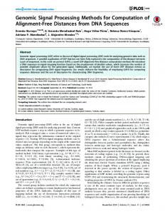
Figure 1: Proximity operator of the function   − ln(ξ − ω) + ln(−ω) if ξ ∈ ]ω, 0] φ : R → ]−∞, +∞] : ξ 7→ − ln(ω − ξ) + ln(ω) if ξ ∈ ]0, ω[   +∞ otherwise.

The proximity operator thresholds over the interval [1/ω, 1/ω], and saturates at −∞ and +∞ with asymptotes at ω and ω, respectively (see Table 2.xiii and [53]).

Proposition 3.7 [16] Assume that, for every y ∈ dom f1 , ∂f1 (y) 6= ∅, and let x be a solution to Problem 3.1. Then every sequence (xn )n∈N generated by Algorithm 3.6 satisfies (∀n ∈ N r {0})

f1 (xn ) + f2 (xn ) ≤ f1 (x) + f2 (x) +

2βkx0 − xk2 . (n + 1)2

(23)

Other variations of the forward-backward algorithm have also been reported to yield improved convergence profiles [20, 70, 97, 134, 135]. Problem 3.1 and Proposition 3.3 cover a wide variety of signal processing problems and solution methods [55]. For the sake of illustration, let us provide a few examples. For notational convenience, we set λn ≡ 1 in Algorithm 3.2, which reduces the updating rule to (17). Example 3.8 (projected gradient) In Problem 3.1, suppose that f1 = ιC , where C is a closed convex subset of RN such that {x ∈ C | f2 (x) ≤ η} is nonempty and bounded for some η ∈ R. Then we obtain the constrained minimization problem minimize f2 (x). x∈C

6

(24)

Since proxγf1 = PC (see Table 1.xii), the forward-backward iteration reduces to the projected gradient method
xn+1 = PC xn − γn ∇f2 (xn ) , ε ≤ γn ≤ 2/β − ε. (25)

This algorithm has been used in numerous signal processing problems, in particular in total variation denoising [34], in image deblurring [18], in pulse shape design [50], and in compressed sensing [73]. Example 3.9 (projected Landweber) In Example 3.8, setting f2 : x 7→ kLx − yk2/2, where L ∈ RM×N r {0} and y ∈ RM , yields the constrained least-squares problem minimize x∈C

1 kLx − yk2 . 2

(26)

Since ∇f2 : x 7→ L⊤ (Lx − y) has Lipschitz constant β = kLk2, (25) yields the projected Landweber method [68]
(27) xn+1 = PC xn + γn L⊤ (y − Lxn ) , ε ≤ γn ≤ 2/kLk2 − ε. This method has been used in particular in computer vision [89] and in signal restoration [129].

Example 3.10 (backward-backward algorithm) Let f and g be functions in Γ0 (RN ). Consider the problem minimize f (x) + ge(x), (28) x∈RN

where e g is the Moreau envelope of g (see Table 1.vii), and suppose that f (x) + ge(x) → +∞ as kxk → +∞. This is a special case of Problem 3.1 with f1 = f and f2 = ge. Since ∇f2 : x 7→ x − proxg x has Lipschitz constant β = 1 [55, 102], Proposition 3.3 with γn ≡ 1 asserts that the sequence (xn )n∈N generated by the backward-backward algorithm xn+1 = proxf (proxg xn )

(29)

converges to a solution to (28). Detailed analyses of this scheme can be found in [1, 14, 48, 108]. Example 3.11 (alternating projections) In Example 3.10, let f and g be respectively the indicator functions of nonempty closed convex sets C and D, one of which is bounded. Then (28) amounts to finding a signal x in C at closest distance from D, i.e., minimize x∈C

1 2 d (x). 2 D

(30)

Moreover, since proxf = PC and proxg = PD , (29) yields the alternating projection method xn+1 = PC (PD xn ),

(31)

which was first analyzed in this context in [41]. Signal processing applications can be found in the areas of spectral estimation [80], pulse shape design [107], wavelet construction [109], and signal synthesis [140]. Example 3.12 (iterative thresholding) Let (bk )1≤k≤N be an orthonormal basis of RN , let (ωk )1≤k≤N be strictly positive real numbers, let L ∈ RM×N r {0}, and let y ∈ RM . Consider the ℓ1 –ℓ2 problem N X 1 (32) minimize ωk |x⊤ bk | + kLx − yk2 . 2 x∈RN k=1

7

D

b

x0

x1 x∞ C

D

y0 y1

y2

b

z0 = x0

x2 z2 z1 = x1

b

b

b

x∞

C

Figure 2: Forward-backward versus Beck-Teboulle : As in Example 3.11, let C and D be two closed convex sets and consider the problem (30) of finding a point x∞ in C at minimum distance from D. Let us set f1 = ιC and f2 = d2D /2. Top: The forward-backward algorithm with γn ≡ 1.9 and λn ≡ 1. As seen in Example 3.11, it reduces to the alternating projection method (31). Bottom: The Beck-Teboulle algorithm.

8

This type of formulation arises in signal recovery problems in which y is the observed signal and the original signal is known to have a sparse representation in the basis (bk )1≤k≤N , e.g., [17, 20, 56, 58, 72, 73, 125, 127]. We observe that (32) is a special case of (15) with ( P f1 : x 7→ 1≤k≤N ωk |x⊤ bk | (33) f2 : x 7→ kLx − yk2 /2.

P ⊤ Since proxγf1 : x 7→ 1≤k≤N soft[−γωk ,γωk ] (x bk ) bk (see Table 1.viii and Table 2.ii), it follows from Proposition 3.3 that the sequence (xn )n∈N generated by the iterative thresholding algorithm xn+1 =

N X

ξk,n bk ,

where

k=1

(


⊤ ξk,n = soft[−γn ωk ,γn ωk ] xn + γn L⊤ (y − Lxn ) bk ε ≤ γn ≤ 2/kLk2 − ε,

(34)

converges to a solution to (32). Additional applications of the forward-backward algorithm in signal and image processing can be found in [30, 28, 29, 32, 36, 37, 53, 55, 57, 74].

4

Douglas-Rachford splitting

The forward-backward algorithm of Section 3 requires that one of the functions be differentiable, with a Lipschitz continuous gradient. In this section, we relax this assumption. Problem 4.1 Let f1 and f2 be functions in Γ0 (RN ) such that (ri dom f1 ) ∩ (ri dom f2 ) 6= ∅

(35)

and f1 (x) + f2 (x) → +∞ as kxk → +∞. The problem is to minimize f1 (x) + f2 (x). x∈RN

(36)

What is nowadays referred to as the Douglas-Rachford algorithm goes back to a method originally proposed in [60] for solving matrix equations of the form u = Ax + Bx, where A and B are positive-definite matrices (see also [132]). The method was transformed in [95] to handle nonlinear problems and further improved in [96] to address monotone inclusion problems. For further developments, see [48, 49, 66]. Problem 4.1 admits at least one solution and, for any γ ∈ ]0, +∞[, its solutions are characterized by the two-level condition [52] ( x = proxγf2 y (37) proxγf2 y = proxγf1 (2proxγf2 y − y), which motivates the following scheme. Algorithm 4.2 (Douglas-Rachford algorithm) Fix ε ∈ ]0, 1[, γ > 0, y0 ∈ RN For n= 0, 1, . . .  xn = proxγf2 yn   λn ∈ [ε, 2 − ε]

yn+1 = yn + λn proxγf1 2xn − yn − xn .

9

(38)

Proposition 4.3 [52] Every sequence (xn )n∈N generated by Algorithm 4.2 converges to a solution to Problem 4.1. Just like the forward-backward algorithm, the Douglas-Rachford algorithm operates by splitting since it employs the functions f1 and f2 separately. It can be viewed as more general in scope than the forward-backward algorithm in that it does not require that any of the functions have a Lipschitz continuous gradient. However, this observation must be weighed against the fact that it may be more demanding numerically as it requires the implementation of two proximal steps at each iteration, whereas only one is needed in the forward-backward algorithm. In some problems, both may be easily implementable (see Fig. 3 for an example) and it is not clear a priori which algorithm may be more efficient. Applications of the Douglas-Rachford algorithm to signal and image processing can be found in [38, 52, 62, 63, 117, 118, 123]. The limiting case of the Douglas-Rachford algorithm in which λn ≡ 2 is the PeacemanRachford algorithm [48, 66, 96]. Its convergence requires additional assumptions (for instance, that f2 be strictly convex and real-valued) [49].

5

Dykstra-like splitting

In this section we consider problems involving a quadratic term penalizing the deviation from a reference signal r. Problem 5.1 Let f and g be functions in Γ0 (RN ) such that dom f ∩ dom g 6= ∅, and let r ∈ RN . The problem is to 1 minimize f (x) + g(x) + kx − rk2 . 2 x∈RN

(39)

It follows at once from (9) that Problem 5.1 admits a unique solution, namely x = proxf +g r. Unfortunately, the proximity operator of the sum of two functions is usually intractable. To compute it iteratively, we can observe that (39) can be viewed as an instance of (36) in Problem 4.1 with f1 = f and f2 = g + k · −rk2/2. However, in this Douglas-Rachford framework, the additional qualification condition (35) needs to be imposed. In the present setting we require only the minimal feasibility condition dom f ∩ dom g 6= ∅. Algorithm 5.2 (Dykstra-like proximal algorithm) Set x0 = r, p0 = 0, q0 = 0 For n = 0, 1, . . .   yn = proxg (xn + pn )   pn+1 = xn + pn − yn   xn+1 = prox (yn + qn ) f qn+1 = yn + qn − xn+1 .

(40)

Proposition 5.3 [12] Every sequence (xn )n∈N generated by Algorithm 5.2 converges to the solution to Problem 5.1. Example 5.4 (best approximation) Let f and g be the indicator functions of closed convex sets C and D, respectively, in Problem 5.1. Then the problem is to find the best approximation to r from C ∩ D, i.e., the projection of r onto C ∩ D. In this case, since proxf = PC and proxg = PD , the above algorithm reduces to Dykstra’s projection method [22, 64]. Example 5.5 (denoising) Consider the problem of recovering a signal x from a noisy observation r = x + w, where w models noise. If f and g are functions in Γ0 (RN ) promoting certain properties of x, adopting a least-squares data fitting objective leads to the variational denoising problem (39).

10

D

b

x0

x2 x3

x1

b

x∞ b

b

C

D x0 b

x1

b

y0

b

x2 y1

b

x3

b b

b b b

y2

b

y3

x4

y4

b

b

b

x∞

C

Figure 3: Forward-backward versus Douglas-Rachford: As in Example 3.11, let C and D be two closed convex sets and consider the problem (30) of finding a point x∞ in C at minimum distance from D. Let us set f1 = ιC and f2 = d2D /2. Top: The forward-backward algorithm with γn ≡ 1 and λn ≡ 1. As seen in Example 3.11, it assumes the form of the alternating projection method (31). Bottom: The Douglas-Rachford algorithm with γ = 1 and λn ≡ 1. Table 1.xii yields proxf1 = PC and Table 1.vi yields proxf2 : x 7→ (x + PD x)/2. Therefore the updating rule in Algorithm 4.2 reduces to xn = (yn + PD yn )/2 and yn+1 = PC (2xn − yn ) + yn − xn = PC (PD yn ) + yn − xn .

11

6

Composite problems

We focus on variational problems with m = 2 functions involving explicitly a linear transformation. Problem 6.1 Let f ∈ Γ0 (RN ), let g ∈ Γ0 (RM ), and let L ∈ RM×N r {0} be such that dom g ∩ L(dom f ) 6= ∅ and f (x) + g(Lx) → +∞ as kxk → +∞. The problem is to minimize f (x) + g(Lx). x∈RN

(41)

Our assumptions guarantee that Problem 6.1 possesses at least one solution. To find such a solution, several scenarios can be contemplated.

6.1

Forward-backward splitting

Suppose that in Problem 6.1 g is differentiable with a τ -Lipschitz continuous gradient (see (14)). Now set f1 = f and f2 = g ◦ L. Then f2 is differentiable and its gradient ∇f2 = L⊤ ◦ ∇g ◦ L

(42)

is β-Lipschitz continuous, with β = τ kLk2 . Hence, we can apply the forward-backward splitting method, as implemented in Algorithm 3.2. As seen in (20), it operates with the updating rule   γn ∈ [ε, 2/(τ kLk2) − ε]   yn = xn − γn L⊤ ∇g(Lxn )  (43)  λn ∈ [ε, 1] xn+1 = xn + λn (proxγn f yn − xn ).

Convergence is guaranteed by Proposition 3.3.

6.2

Douglas-Rachford splitting

Suppose that in Problem 6.1 the matrix L satisfies LL⊤ = νI,

where ν ∈ ]0, +∞[

(44)

and (ri dom g) ∩ ri L(dom f ) 6= ∅. Let us set f1 = f and f2 = g ◦ L. As seen in Table 1.x, proxf2 has a closed-form expression in terms of proxg and we can therefore apply the Douglas-Rachford splitting method (Algorithm 4.2). In this scenario, the updating rule reads
  xn = yn + ν −1 L⊤ proxγνg (Lyn ) − Lyn   λn ∈ [ε, 2 − ε] (45)

yn+1 = yn + λn proxγf 2xn − yn − xn . Convergence is guaranteed by Proposition 4.3.

6.3

Dual forward-backward splitting

Suppose that in Problem 6.1 f = h + k · −rk2 /2, where h ∈ Γ0 (RN ) and r ∈ RN . Then (41) becomes 1 (46) minimize h(x) + g(Lx) + kx − rk2 , N 2 x∈R which models various signal recovery problems, e.g., [33, 34, 51, 59, 112, 138]. If (44) holds, proxg◦L is decomposable, and (46) can be solved with the Dykstra-like method of Section 5, where f1 = h + k · −rk2 /2 (see Table 1.iv) and f2 = g ◦ L (see Table 1.x). Otherwise, we can exploit the nice properties of the Fenchel-Moreau-Rockafellar dual of (46), solve this dual problem by forward-backward splitting, and recover the unique solution to (46) [51].

12

Algorithm 6.2 (Dual forward-backward algorithm)   Fix ε ∈ 0, min{1, 1/kLk2} , u0 ∈ RM For n = 0, 1, . . .   xn = proxh (r − L⊤ un )      γn ∈ ε, 2/kLk2 − ε   λn ∈ [ε, 1]
un+1 = un + λn proxγn g∗ (un + γn Lxn ) − un .

(47)

Proposition 6.3 [51] Assume that (ri dom g)∩ri L(dom h) 6= ∅. Then every sequence (xn )n∈N generated by the dual forward-backward algorithm 6.2 converges to the solution to (46).

6.4

Alternating-direction method of multipliers

Augmented Lagrangian techniques are classical approaches for solving Problem 6.1 [77, 78] (see also [75, 79]). First, observe that (41) is equivalent to minimize f (x) + g(y).

x∈RN , y∈RM Lx=y

(48)

The augmented Lagrangian of index γ ∈ ]0, +∞[ associated with (48) is the saddle function Lγ : RN × RM × RM → ]−∞, +∞] (x, y, z) 7→ f (x) + g(y) +

1 1 ⊤ z (Lx − y) + kLx − yk2 . γ 2γ

(49)

The alternating-direction method of multipliers consists in minimizing Lγ over x, then over y, and then applying a proximal maximization step with respect to the Lagrange multiplier z. Now suppose that L⊤ L is invertible and (ri dom g) ∩ ri L(dom f ) 6= ∅.

(50)

M By analogy with (9), if we denote by proxL to the f the operator which maps a point y ∈ R 2 unique minimizer of x 7→ f (x) + kLx − yk /2, we obtain the following implementation.

Algorithm 6.4 (Alternating-direction method of multipliers (ADMM)) Fix γ > 0, y0 ∈ RM , z0 ∈ RM For n =0, 1, . . .  x = proxL (y − z ) n  n γf n   sn = Lxn   yn+1 = proxγg (sn + zn ) zn+1 = zn + sn − yn+1 .

(51)

The convergence of the sequence (xn )n∈N thus produced under assumption (50) has been investigated in several places, e.g., [75, 77, 79]. It was first observed in [76] that the ADMM algorithm can be derived from an application of the Douglas-Rachford algorithm to the dual of (41). This analysis was pursued in [66], where the convergence of (xn )n∈N to a solution to (41) is shown. Variants of the method relaxing the requirements on L in (50) have been proposed [5, 39]. In image processing, ADMM was applied in [81] to an ℓ1 regularization problem under the name “alternating split Bregman algorithm.” Further applications and connections are found in [2, 69, 117, 143].

13

7

Problems with m ≥ 2 functions

We return to the general minimization problem (1). Problem 7.1 Let f1 ,. . . ,fm be functions in Γ0 (RN ) such that (ri dom f1 ) ∩ · · · ∩ (ri dom fm ) 6= ∅

(52)

and f1 (x) + · · · + fm (x) → +∞ as kxk → +∞. The problem is to minimize f1 (x) + · · · + fm (x). x∈RN

(53)

Since the methods described so far are designed for m = 2 functions, we can attempt to reformulate (53) as a 2-function problem in the m-fold product space H = RN × · · · × RN

(54)

(such techniques were introduced in [110, 111] and have been used in the context of convex feasibility problems in [10, 43, 45]). To this end, observe that (53) can be rewritten in H as minimize

(x1 ,...,xm )∈H x1 =···=xm

f1 (x1 ) + · · · + fm (xm ).

(55)

If we denote by x = (x1 , . . . , xm ) a generic element in H, (55) is equivalent to minimize ιD (x) + f (x),

(56)

 D = (x, . . . , x) ∈ H | x ∈ RN f : x 7→ f1 (x1 ) + · · · + fm (xm ).

(57)

x∈H

where

(

We are thus back to a problem involving two functions in the larger space H. In some cases, this observation makes it possible to obtain convergent methods from the algorithms discussed in the preceding sections. For instance, the following parallel algorithm was derived from the Douglas-Rachford algorithm in [54] (see also [49] for further analysis and connections with Spingarn’s splitting method [120]). Algorithm 7.2 (Parallel proximal algorithm (PPXA)) m Fix ε ∈ ]0, 1[, γ > 0, (ωi )1≤i≤m ∈ ]0, 1] such that Pm N N i=1 ωi = 1, y1,0 ∈ R , . . . , ym,0 ∈ R Pm Set x0 = i=1 ωi yi,0 For  n = 0, 1, . . .  For i = 1, . . . , m  j   pi,n = proxγfi /ωi yi,n  m  X   pn = ωi pi,n   i=1  ε≤λ ≤2−ε n    For i = 1, . . . , m
  yi,n+1 = yi,n + λn 2pn − xn − pi,n  xn+1 = xn + λn (pn − xn ). Proposition 7.3 [54] Every sequence (xn )n∈N generated by Algorithm 7.2 converges to a solution to Problem 7.1.

14

Example 7.4 (image recovery) In many imaging problems, we record an observation y ∈ RM of an image z ∈ RK degraded by a matrix L ∈ RM×K and corrupted by noise. In the spirit of a number of recent investigations (see [37] and the references therein), a tight frame representation of the images under consideration can be used. This representation is defined through a synthesis matrix F ⊤ ∈ RK×N (with K ≤ N ) such that F ⊤ F = νI, for some ν ∈ ]0, +∞[. Thus, the original image can be written as z = F ⊤ x, where x ∈ RN is a vector of frame coefficients to be estimated. For this purpose, we consider the problem minimize x∈C

1 kLF ⊤ x − yk2 + Φ(x) + tv(F ⊤ x), 2

(58)

where C is a closed convex set modeling a constraint on z, the quadratic term is the standard least-squares data fidelity term, Φ is a real-valued convex function on RN (e.g., a weighted ℓ1 norm) introducing a regularization on the frame coefficients, and tv is a discrete total variation function aiming at preserving piecewise smooth areas and sharp edges [116]. Using appropriate gradient filters in the computation of tv, it is possible to decompose it as a sum of convex functions (tvi )1≤i≤q , the proximity operators of which can be expressed in closed form [54, 113]. Thus, (58) appears as a special case of (53) with m = q + 3, f1 = ιC , f2 = kLF ⊤ · −yk2 /2, f3 = Φ, and f3+i = tvi (F ⊤ ·) for i ∈ {1, . . . , q}. Since a tight frame is employed, the proximity operators of f2 and (f3+i )1≤i≤q can be deduced from Table 1.x. Thus, the PPXA algorithm is well suited for solving this problem numerically. A product space strategy can also be adopted to address the following extension of Problem 5.1. Problem 7.5 Let f1 , . . . , fm be functions in Γ0 (RN ) such that dom f1 ∩ · · · ∩ dom fm 6= ∅, Pm m let (ωi )1≤i≤m ∈ ]0, 1] be such that i=1 ωi = 1, and let r ∈ RN . The problem is to minimize x∈RN

m X

1 ωi fi (x) + kx − rk2 . 2 i=1

Algorithm 7.6 (Parallel Dykstra-like proximal algorithm) Set x0 = r, z1,0 = x0 , . . . , zm,0 = x0 For n= 0, 1, . . .  For i = 1, . . . , m    pi,n = prox zi,n fi  P   xn+1 = m i=1 ωi pi,n   For i = 1, . . . , m   zi,n+1 = xn+1 + zi,n − pi,n .

(59)

(60)

Proposition 7.7 [49] Every sequence (xn )n∈N generated by Algorithm 7.6 converges to the solution to Problem 7.5. Next, we consider a composite problem. Problem 7.8 For every i ∈ {1, . . . , m}, let gi ∈ Γ0 (RMi ) and let Li ∈ RMi ×N . Assume that (∃ q ∈ RN ) L1 q ∈ ri dom g1 , . . . , Lm q ∈ ri dom gm , (61) P that g1 (L1 x) + · · · + gm (Lm x) → +∞ as kxk → +∞, and that Q = 1≤i≤m L⊤ i Li is invertible. The problem is to minimize g1 (L1 x) + · · · + gm (Lm x). (62) x∈RN

15

Proceeding as in (55) and (56), (62) can be recast as minimize ιD (x) + g(y), x∈H, y∈G y=Lx

where

 Mm N N M1  H = R × · · · × R , G = R × · · · × R L : H → G : x 7→ (L1 x1 , . . . , Lm xm )   g : G → ]−∞, +∞] : y 7→ g1 (y1 ) + · · · + gm (ym ).

(63)

(64)

In turn, a solution to (62) can be obtained as the limit of the sequence (xn )n∈N constructed by the following algorithm, which can be derived from the alternating-direction method of multipliers of Section 6.4 (alternative parallel offsprings of ADMM exist, see for instance [65]). Algorithm 7.9 (Simultaneous-direction method of multipliers (SDMM)) Fix γ > 0, y1,0 ∈ RM1 , . . . , ym,0 ∈ RMm , z1,0 ∈ RM1 , . . . , zm,0 ∈ RMm For n = 0, 1, . . .  P ⊤  xn = Q−1 m i=1 Li (yi,n − zi,n )   For i = 1, . . . , m     si,n = Li xn     y   i,n+1 = proxγgi (si,n + zi,n ) zi,n+1 = zi,n + si,n − yi,n+1

(65)

This algorithm was derived from a slightly different viewpoint in [118] with a connection with the work of [71]. In these papers, SDMM is applied to deblurring in the presence of Poisson noise. The computation of xn in (65) requires the solution of a positive-definite symmetric system of linear equations. Efficient methods for solving such systems can be found in [82]. In certain situations, fast Fourier diagonalization is also an option [2, 71]. In the above algorithms, the proximal vectors, as well as the auxiliary vectors, can be computed simultaneously at each iteration. This parallel structure is useful when the algorithms are implemented on multicore architectures. A parallel proximal algorithm is also available to solve multicomponent signal processing problems [27]. This framework captures in particular problem formulations found in [7, 8, 80, 88, 133]. Let us add that an alternative splitting framework applicable to (53) was recently proposed in [67].

8

Conclusion

We have presented a panel of convex optimization algorithms sharing two main features. First, they employ proximity operators, a powerful generalization of the notion of a projection operator. Second, they operate by splitting the objective to be minimized into simpler functions that are dealt with individually. These methods are applicable to a wide class of signal and image processing problems ranging from restoration and reconstruction to synthesis and design. One of the main advantages of these algorithms is that they can be used to minimize nondifferentiable objectives, such as those commonly encountered in sparse approximation and compressed sensing, or in hard-constrained problems. Finally, let us note that the variational problems described in (39), (46), and (59), consist of computing a proximity operator. Therefore the associated algorithms can be used as a subroutine to compute approximately proximity operators within a proximal splitting algorithm, provided the latter is error tolerant (see [48, 49, 51, 66, 115] for convergence properties under approximate proximal computations). An application of this principle can be found in [38].

16

References [1] Acker, F., Prestel, M.A.: Convergence d’un sch´ema de minimisation altern´ee. Ann. Fac. Sci. Toulouse V. S´er. Math. 2, 1–9 (1980) [2] Afonso, M.V., Bioucas-Dias, J.M., Figueiredo, M.A.T.: Fast image recovery using variable splitting and constrained optimization (2009). http://arxiv.org/abs/0910.4887 [3] Antoniadis, A., Fan, J.: Regularization of wavelet approximations. J. Amer. Statist. Assoc. 96, 939–967 (2001) [4] Antoniadis, A., Leporini, D., Pesquet, J.C.: Wavelet thresholding for some classes of non-Gaussian noise. Statist. Neerlandica 56, 434–453 (2002) [5] Attouch, H., Soueycatt, M.: Augmented Lagrangian and proximal alternating direction methods of multipliers in Hilbert spaces – applications to games, PDEs and control. Pacific J. Optim. 5, 17–37 (2009) [6] Aubin, J.P.: Optima and Equilibria – An Introduction to Nonlinear Analysis, 2nd edn. Springer-Verlag, New York (1998) [7] Aujol, J.F., Aubert, G., Blanc-F´eraud, L., Chambolle, A.: Image decomposition into a bounded variation component and an oscillating component. J. Math. Imaging Vision 22, 71–88 (2005) [8] Aujol, J.F., Chambolle, A.: Dual norms and image decomposition models. Int. J. Computer Vision 63, 85–104 (2005) [9] Bauschke, H.H., Borwein, J.M.: Dykstra’s alternating projection algorithm for two sets. J. Approx. Theory 79, 418–443 (1994) [10] Bauschke, H.H., Borwein, J.M.: On projection algorithms for solving convex feasibility problems. SIAM Rev. 38, 367–426 (1996) [11] Bauschke, H.H., Combettes, P.L.: A weak-to-strong convergence principle for Fej´ermonotone methods in Hilbert spaces. Math. Oper. Res. 26, 248–264 (2001) [12] Bauschke, H.H., Combettes, P.L.: A Dykstra-like algorithm for two monotone operators. Pacific J. Optim. 4, 383–391 (2008) [13] Bauschke, H.H., Combettes, P.L.: Convex Analysis and Monotone Operator Theory in Hilbert Spaces. Springer-Verlag (2011). To appear [14] Bauschke, H.H., Combettes, P.L., Reich, S.: The asymptotic behavior of the composition of two resolvents. Nonlinear Anal. 60, 283–301 (2005) [15] Beck, A., Teboulle, M.: Fast gradient-based algorithms for constrained total variation image denoising and deblurring problems. IEEE Trans. Image Process. 18, 2419–2434 (2009) [16] Beck, A., Teboulle, M.: A fast iterative shrinkage-thresholding algorithm for linear inverse problems. SIAM J. Imaging Sci. 2, 183–202 (2009) [17] Bect, J., Blanc-F´eraud, L., Aubert, G., Chambolle, A.: A ℓ1 unified variational framework for image restoration. Lecture Notes in Comput. Sci. 3024, 1–13 (2004) [18] Benvenuto, F., Zanella, R., Zanni, L., Bertero, M.: Nonnegative least-squares image deblurring: improved gradient projection approaches. Inverse Problems 26, 18 (2010). Art. 025004 [19] Bertsekas, D.P., Tsitsiklis, J.N.: Parallel and Distributed Computation: Numerical Methods. Athena Scientific, Belmont, MA (1997) [20] Bioucas-Dias, J.M., Figueiredo, M.A.T.: A new TwIST: Two-step iterative shrinkage/thresholding algorithms for image restoration. IEEE Trans. Image Process. 16, 2992–3004 (2007)

17

[21] Bouman, C., Sauer, K.: A generalized Gaussian image model for edge-preserving MAP estimation. IEEE Trans. Image Process. 2, 296–310 (1993) [22] Boyle, J.P., Dykstra, R.L.: A method for finding projections onto the intersection of convex sets in Hilbert spaces. Lecture Notes in Statist. 37, 28–47 (1986) [23] Bredies, K.: A forward-backward splitting algorithm for the minimization of non-smooth convex functionals in Banach space. Inverse Problems 25, 20 (2009). Art. 015005 [24] Bredies, K., Lorenz, D.A.: Linear convergence of iterative soft-thresholding. J. Fourier Anal. Appl. 14, 813–837 (2008) [25] Br`egman, L.M.: The method of successive projection for finding a common point of convex sets. Soviet Math. Dokl. 6, 688–692 (1965) [26] Br´ezis, H., Lions, P.L.: Produits infinis de r´esolvantes. Israel J. Math. 29, 329–345 (1978) [27] Brice˜ no-Arias, L.M., Combettes, P.L.: Convex variational formulation with smooth coupling for multicomponent signal decomposition and recovery. Numer. Math. Theory Methods Appl. 2, 485–508 (2009) [28] Cai, J.F., Chan, R.H., Shen, L., Shen, Z.: Convergence analysis of tight framelet approach for missing data recovery. Adv. Comput. Math. 31, 87–113 (2009) [29] Cai, J.F., Chan, R.H., Shen, L., Shen, Z.: Simultaneously inpainting in image and transformed domains. Numer. Math. 112, 509–533 (2009) [30] Cai, J.F., Chan, R.H., Shen, Z.: A framelet-based image inpainting algorithm. Appl. Comput. Harm. Anal. 24, 131–149 (2008) [31] Censor, Y., Zenios, S.A.: Parallel Optimization: Theory, Algorithms and Applications. Oxford University Press, New York (1997) [32] Chaˆari, L., Pesquet, J.C., Ciuciu, P., Benazza-Benyahia, A.: An iterative method for parallel MRI SENSE-based reconstruction in the wavelet domain (2009). http://wwwsyscom.univ-mlv.fr/∼chaari/downloads/MEDIA Chaari.pdf [33] Chambolle, A.: An algorithm for total variation minimization and applications. J. Math. Imaging Vision 20, 89–97 (2004) [34] Chambolle, A.: Total variation minimization and a class of binary MRF model. Lecture Notes in Comput. Sci. 3757, 136–152 (2005) [35] Chambolle, A., DeVore, R.A., Lee, N.Y., Lucier, B.J.: Nonlinear wavelet image processing: Variational problems, compression, and noise removal through wavelet shrinkage. IEEE Trans. Image Process. 7, 319–335 (1998) [36] Chan, R.H., Setzer, S., Steidl, G.: Inpainting by flexible Haar-wavelet shrinkage. SIAM J. Imaging Sci. 1, 273–293 (2008) [37] Chaux, C., Combettes, P.L., Pesquet, J.C., Wajs, V.R.: A variational formulation for frame-based inverse problems. Inverse Problems 23, 1495–1518 (2007) [38] Chaux, C., Pesquet, J.C., Pustelnik, N.: Nested iterative algorithms for convex constrained image recovery problems. SIAM J. Imaging Sci. 2, 730–762 (2009) [39] Chen, G., Teboulle, M.: A proximal-based decomposition method for convex minimization problems. Math. Programming 64, 81–101 (1994) [40] Chen, G.H.G., Rockafellar, R.T.: Convergence rates in forward-backward splitting. SIAM J. Optim. 7, 421–444 (1997) [41] Cheney, W., Goldstein, A.A.: Proximity maps for convex sets. Proc. Amer. Math. Soc. 10, 448–450 (1959) [42] Combettes, P.L.: The foundations of set theoretic estimation. Proc. IEEE 81, 182–208 (1993) [43] Combettes, P.L.: Inconsistent signal feasibility problems: Least-squares solutions in a product space. IEEE Trans. Signal Process. 42, 2955–2966 (1994)

18

[44] Combettes, P.L.: The convex feasibility problem in image recovery. In: P. Hawkes (ed.) Advances in Imaging and Electron Physics, vol. 95, pp. 155–270. Academic Press, New York (1996) [45] Combettes, P.L.: Convex set theoretic image recovery by extrapolated iterations of parallel subgradient projections. IEEE Trans. Image Process. 6, 493–506 (1997) [46] Combettes, P.L.: Convexit´e et signal. In: Proc. Congr`es de Math´ematiques Appliqu´ees et Industrielles SMAI’01, pp. 6–16. Pompadour, France (2001) [47] Combettes, P.L.: A block-iterative surrogate constraint splitting method for quadratic signal recovery. IEEE Trans. Signal Process. 51, 1771–1782 (2003) [48] Combettes, P.L.: Solving monotone inclusions via compositions of nonexpansive averaged operators. Optimization 53, 475–504 (2004) [49] Combettes, P.L.: Iterative construction of the resolvent of a sum of maximal monotone operators. J. Convex Anal. 16, 727–748 (2009) [50] Combettes, P.L., Bondon, P.: Hard-constrained inconsistent signal feasibility problems. IEEE Trans. Signal Process. 47, 2460–2468 (1999) [51] Combettes, P.L., D˜ ung, D., V˜ u, B.C.: Dualization of signal recovery problems (2009). http://arxiv.org/abs/0907.0436 [52] Combettes, P.L., Pesquet, J.C.: A Douglas-Rachford splitting approach to nonsmooth convex variational signal recovery. IEEE J. Selected Topics Signal Process. 1, 564–574 (2007) [53] Combettes, P.L., Pesquet, J.C.: Proximal thresholding algorithm for minimization over orthonormal bases. SIAM J. Optim. 18, 1351–1376 (2007) [54] Combettes, P.L., Pesquet, J.C.: A proximal decomposition method for solving convex variational inverse problems. Inverse Problems 24, 27 (2008). Art. 065014 [55] Combettes, P.L., Wajs, V.R.: Signal recovery by proximal forward-backward splitting. Multiscale Model. Simul. 4, 1168–1200 (2005) [56] Daubechies, I., Defrise, M., De Mol, C.: An iterative thresholding algorithm for linear inverse problems with a sparsity constraint. Comm. Pure Appl. Math. 57, 1413–1457 (2004) [57] Daubechies, I., Teschke, G., Vese, L.: Iteratively solving linear inverse problems under general convex constraints. Inverse Probl. Imaging 1, 29–46 (2007) [58] De Mol, C., Defrise, M.: A note on wavelet-based inversion algorithms. Contemp. Math. 313, 85–96 (2002) [59] Didas, S., Setzer, S., Steidl, G.: Combined ℓ2 data and gradient fitting in conjunction with ℓ1 regularization. Adv. Comput. Math. 30, 79–99 (2009) [60] Douglas, J., Rachford, H.H.: On the numerical solution of heat conduction problems in two or three space variables. Trans. Amer. Math. Soc. 82, 421–439 (1956) [61] Dunn, J.C.: Convexity, monotonicity, and gradient processes in Hilbert space. J. Math. Anal. Appl. 53, 145–158 (1976) [62] Dup´e, F.X., Fadili, M.J., Starck, J.L.: A proximal iteration for deconvolving Poisson noisy images using sparse representations. IEEE Trans. Image Process. 18, 310–321 (2009) [63] Durand, S., Fadili, J., Nikolova, M.: Multiplicative noise removal using L1 fidelity on frame coefficients. J. Math. Imaging Vision 36, 201–226 (2010) [64] Dykstra, R.L.: An algorithm for restricted least squares regression. J. Amer. Stat. Assoc. 78, 837–842 (1983) [65] Eckstein, J.: Parallel alternating direction multiplier decomposition of convex programs. J. Optim. Theory Appl. 80, 39–62 (1994)

19

[66] Eckstein, J., Bertsekas, D.P.: On the Douglas-Rachford splitting method and the proximal point algorithm for maximal monotone operators. Math. Programming 55, 293–318 (1992) [67] Eckstein, J., Svaiter, B.F.: General projective splitting methods for sums of maximal monotone operators. SIAM J. Control Optim. 48, 787–811 (2009) [68] Eicke, B.: Iteration methods for convexly constrained ill-posed problems in Hilbert space. Numer. Funct. Anal. Optim. 13, 413–429 (1992) [69] Esser, E.: Applications of Lagrangian-based alternating direction methods and connections to split Bregman (2009). ftp://ftp.math.ucla.edu/pub/camreport/cam09-31.pdf [70] Fadili, J., Peyr´e, G.: Total variation projection with first order schemes (2009). http://hal.archives-ouvertes.fr/hal-00380491 [71] Figueiredo, M.A.T., Bioucas-Dias, J.M.: Deconvolution of Poissonian images using variable splitting and augmented Lagrangian optimization. In: Proc. IEEE Workshop Statist. Signal Process. Cardiff, UK (2009). http://arxiv.org/abs/0904.4872 [72] Figueiredo, M.A.T., Nowak, R.D.: An EM algorithm for wavelet-based image restoration. IEEE Trans. Image Process. 12, 906–916 (2003) [73] Figueiredo, M.A.T., Nowak, R.D., Wright, S.J.: Gradient projection for sparse reconstruction: Application to compressed sensing and other inverse problems. IEEE J. Selected Topics Signal Process. 1, 586–597 (2007) [74] Fornasier, M.: Domain decomposition methods for linear inverse problems with sparsity constraints. Inverse Problems 23, 2505–2526 (2007) [75] Fortin, M., Glowinski, R. (eds.): Augmented Lagrangian Methods: Applications to the Numerical Solution of Boundary-Value Problems. North-Holland, Amsterdam (1983) [76] Gabay, D.: Applications of the method of multipliers to variational inequalities. In: M. Fortin, R. Glowinski (eds.) Augmented Lagrangian Methods: Applications to the Numerical Solution of Boundary-Value Problems, pp. 299–331. North-Holland, Amsterdam (1983) [77] Gabay, D., Mercier, B.: A dual algorithm for the solution of nonlinear variational problems via finite elements approximations. Comput. Math. Appl. 2, 17–40 (1976) [78] Glowinski, R., Marrocco, A.: Sur l’approximation, par ´el´ements finis d’ordre un, et la r´esolution, par p´enalisation-dualit´e, d’une classe de probl`emes de Dirichlet non lin´eaires. RAIRO Anal. Numer. 2, 41–76 (1975) [79] Glowinski, R., Tallec, P.L. (eds.): Augmented Lagrangian and Operator-Splitting Methods in Nonlinear Mechanics. SIAM, Philadelphia (1989) [80] Goldburg, M., Marks II, R.J.: Signal synthesis in the presence of an inconsistent set of constraints. IEEE Trans. Circuits Syst. 32, 647–663 (1985) [81] Goldstein, T., Osher, S.: The split Bregman method for L1-regularized problems. SIAM J. Imaging Sci. 2, 323–343 (2009) [82] Golub, G.H., Van Loan, C.F.: Matrix Computations, 3rd edn. Johns Hopkins University Press, Baltimore, MD (1996) [83] G¨ uler, O.: On the convergence of the proximal point algorithm for convex minimization. SIAM J. Control Optim. 20, 403–419 (1991) [84] G¨ uler, O.: New proximal point algorithms for convex minimization. SIAM J. Optim. 2, 649–664 (1992) [85] Hale, E.T., Yin, W., Zhang, Y.: Fixed-point continuation for l1 -minimization: methodology and convergence. SIAM J. Optim. 19, 1107–1130 (2008) [86] Herman, G.T.: Fundamentals of Computerized Tomography – Image Reconstruction from Projections, 2nd edn. Springer-Verlag, London (2009)

20

[87] Hiriart-Urruty, J.B., Lemar´echal, C.: Fundamentals of Convex Analysis. Springer-Verlag, New York (2001) [88] Huang, Y., Ng, M.K., Wen, Y.W.: A fast total variation minimization method for image restoration. Multiscale Model. Simul. 7, 774–795 (2008) [89] Johansson, B., Elfving, T., Kozlovc, V., Censor, Y., Forss´en, P.E., Granlund, G.: The application of an oblique-projected Landweber method to a model of supervised learning. Math. Comput. Modelling 43, 892–909 (2006) [90] Kiwiel, K.C., Lopuch, B.: Surrogate projection methods for finding fixed points of firmly nonexpansive mappings. SIAM J. Optim. 7, 1084–1102 (1997) [91] Lemaire, B.: The proximal algorithm. In: J.P. Penot (ed.) New Methods in Optimization and Their Industrial Uses, International Series of Numerical Mathematics, vol. 87, pp. 73–87. Birkh¨ auser, Boston, MA (1989) ´ [92] Lemaire, B.: It´eration et approximation. In: Equations aux D´eriv´ees Partielles et Applications, pp. 641–653. Gauthiers-Villars, Paris (1998) [93] Lent, A., Tuy, H.: An iterative method for the extrapolation of band-limited functions. J. Math. Anal. Appl. 83, 554–565 (1981) [94] Levitin, E.S., Polyak, B.T.: Constrained minimization methods. U.S.S.R. Comput. Math. Math. Phys. 6, 1–50 (1966) [95] Lieutaud, J.: Approximation d’Op´erateurs par des M´ethodes de D´ecomposition. Th`ese, Universit´e de Paris (1969) [96] Lions, P.L., Mercier, B.: Splitting algorithms for the sum of two nonlinear operators. SIAM J. Numer. Anal. 16, 964–979 (1979) [97] Loris, I., Bertero, M., De Mol, C., Zanella, R., Zanni, L.: Accelerating gradient projection methods for ℓ1 -constrained signal recovery by steplength selection rules. Appl. Comput. Harm. Anal. 27, 247–254 (2009) [98] Martinet, B.: R´egularisation d’in´equations variationnelles par approximations successives. Rev. Fran¸caise Informat. Rech. Op´er. 4, 154–158 (1970) [99] Mercier, B.: Topics in Finite Element Solution of Elliptic Problems. No. 63 in Lectures on Mathematics. Tata Institute of Fundamental Research, Bombay (1979) [100] Mercier, B.: In´equations Variationnelles de la M´ecanique. No. 80.01 in Publications Math´ematiques d’Orsay. Universit´e de Paris-XI, Orsay, France (1980) [101] Moreau, J.J.: Fonctions convexes duales et points proximaux dans un espace hilbertien. C. R. Acad. Sci. Paris S´er. A Math. 255, 2897–2899 (1962) [102] Moreau, J.J.: Proximit´e et dualit´e dans un espace hilbertien. Bull. Soc. Math. France 93, 273–299 (1965) [103] Nemirovsky, A.S., Yudin, D.B.: Problem Complexity and Method Efficiency in Optimization. Wiley, New York (1983) [104] Nesterov, Yu.: Smooth minimization of non-smooth functions. Math. Program. 103, 127–152 (2005) [105] Nesterov, Yu.: Gradient methods for minimizing composite objective function. CORE discussion paper 2007076, Universit´e Catholique de Louvain, Center for Operations Research and Econometrics (2007) [106] Nesterov, Yu.E.: A method of solving a convex programming problem with convergence rate o(1/k 2 ). Soviet Math. Dokl. 27, 372–376 (1983) [107] Nobakht, R.A., Civanlar, M.R.: Optimal pulse shape design for digital communication systems by projections onto convex sets. IEEE Trans. Communications 43, 2874–2877 (1995)

21

[108] Passty, G.B.: Ergodic convergence to a zero of the sum of monotone operators in Hilbert space. J. Math. Anal. Appl. 72, 383–390 (1979) [109] Pesquet, J.C., Combettes, P.L.: Wavelet synthesis by alternating projections. IEEE Trans. Signal Process. 44, 728–732 (1996) ´ [110] Pierra, G.: Eclatement de contraintes en parall`ele pour la minimisation d’une forme quadratique. Lecture Notes in Comput. Sci. 41, 200–218 (1976) [111] Pierra, G.: Decomposition through formalization in a product space. Math. Programming 28, 96–115 (1984) [112] Potter, L.C., Arun, K.S.: A dual approach to linear inverse problems with convex constraints. SIAM J. Control Optim. 31, 1080–1092 (1993) [113] Pustelnik, N., Chaux, C., Pesquet, J.C.: Parallel proximal algorithm for image restoration using hybrid regularization (2009). http://arxiv.org/abs/0911.1536 [114] Rockafellar, R.T.: Convex Analysis. Princeton University Press, Princeton, NJ (1970) [115] Rockafellar, R.T.: Monotone operators and the proximal point algorithm. SIAM J. Control Optim. 14, 877–898 (1976) [116] Rudin, L.I., Osher, S., Fatemi, E.: Nonlinear total variation based noise removal algorithms. Physica D 60, 259–268 (1992) [117] Setzer, S.: Split Bregman algorithm, Douglas-Rachford splitting and frame shrinkage. Lecture Notes in Comput. Sci. 5567, 464–476 (2009) [118] Setzer, S., Steidl, G., Teuber, T.: Deblurring Poissonian images by split Bregman techniques. J. Vis. Commun. Image Represent. 21, 193–199 (2010) [119] Sibony, M.: M´ethodes it´eratives pour les ´equations et in´equations aux d´eriv´ees partielles non lin´eaires de type monotone. Calcolo 7, 65–183 (1970) [120] Spingarn, J.E.: Partial inverse of a monotone operator. Appl. Math. Optim. 10, 247–265 (1983) [121] Stark, H. (ed.): Image Recovery: Theory and Application. Academic Press, San Diego, CA (1987) [122] Stark, H., Yang, Y.: Vector Space Projections : A Numerical Approach to Signal and Image Processing, Neural Nets, and Optics. Wiley, New York (1998) [123] Steidl, G., Teuber, T.: Removing multiplicative noise by Douglas-Rachford splitting methods. J. Math. Imaging Vision 36, 168–184 (2010) [124] Thompson, A.M., Kay, J.: On some Bayesian choices of regularization parameter in image restoration. Inverse Problems 9, 749–761 (1993) [125] Tibshirani, R.: Regression shrinkage and selection via the lasso. J. Royal. Statist. Soc. B 58, 267–288 (1996) [126] Titterington, D.M.: General structure of regularization procedures in image reconstruction. Astronom. and Astrophys. 144, 381–387 (1985) [127] Tropp, J.A.: Just relax: Convex programming methods for identifying sparse signals in noise. IEEE Trans. Inform. Theory 52, 1030–1051 (2006) [128] Trussell, H.J., Civanlar, M.R.: The feasible solution in signal restoration. IEEE Trans. Acoust., Speech, Signal Process. 32, 201–212 (1984) [129] Trussell, H.J., Civanlar, M.R.: The Landweber iteration and projection onto convex sets. IEEE Trans. Acoust., Speech, Signal Process. 33, 1632–1634 (1985) [130] Tseng, P.: Applications of a splitting algorithm to decomposition in convex programming and variational inequalities. SIAM J. Control Optim. 29, 119–138 (1991) [131] Tseng, P.: On accelerated proximal gradient methods for convex-concave optimization (2008). http://www.math.washington.edu/∼tseng/papers/apgm.pdf

22

[132] Varga, R.S.: Matrix Iterative Analysis, 2nd edn. Springer-Verlag, New York (2000) [133] Vese, L.A., Osher, S.J.: Image denoising and decomposition with total variation minimization and oscillatory functions. J. Math. Imaging Vision 20, 7–18 (2004) [134] Vonesh, C., Unser, M.: A fast thresholded Landweber algorithm for wavelet-regularized multidimensional deconvolution. IEEE Trans. Image Process. 17, 539–549 (2008) [135] Vonesh, C., Unser, M.: A fast multilevel algorithm for wavelet-regularized image restoration. IEEE Trans. Image Process. 18, 509–523 (2009) [136] Weiss, P., Aubert, G., Blanc-F´eraud, L.: Efficient schemes for total variation minimization under constraints in image processing. SIAM J. Sci. Comput. 31, 2047–2080 (2009) [137] Yamada, I., Ogura, N., Yamashita, Y., Sakaniwa, K.: Quadratic optimization of fixed points of nonexpansive mappings in Hilbert space. Numer. Funct. Anal. Optim. 19, 165–190 (1998) [138] Youla, D.C.: Generalized image restoration by the method of alternating orthogonal projections. IEEE Trans. Circuits Syst. 25, 694–702 (1978) [139] Youla, D.C.: Mathematical theory of image restoration by the method of convex projections. In: H. Stark (ed.) Image Recovery: Theory and Application, pp. 29–77. Academic Press, San Diego, CA (1987) [140] Youla, D.C., Velasco, V.: Extensions of a result on the synthesis of signals in the presence of inconsistent constraints. IEEE Trans. Circuits Syst. 33, 465–468 (1986) [141] Youla, D.C., Webb, H.: Image restoration by the method of convex projections: Part 1 – theory. IEEE Trans. Medical Imaging 1, 81–94 (1982) [142] Zeidler, E.: Nonlinear Functional Analysis and Its Applications, vol. I–V. Springer-Verlag, New York (1985–1990) [143] Zhang, X., Burger, M., Bresson, X., Osher, S.: Bregmanized nonlocal regularization for deconvolution and sparse reconstruction (2009). ftp://ftp.math.ucla.edu/pub/camreport/cam09-03.pdf [144] Zhu, C.Y.: Asymptotic convergence analysis of the forward-backward splitting algorithm. Math. Oper. Res. 20, 449–464 (1995)

23

Table 1: Properties of proximity operators [27, 37, 53, 54, 55, 102]: ϕ ∈ Γ0 (RN ); C ⊂ RN is nonempty, closed, and convex; x ∈ RN . Property f (x) proxf x i ii iii

translation scaling reflection

ϕ(x − z), z ∈ RN ϕ(x/ρ), ρ ∈ R r {0} ϕ(−x)

iv v

quadratic perturbation conjugation

vi

squared distance

ϕ(x) + αkxk2 /2 + u⊤ x + γ u ∈ RN , α ≥ 0, γ ∈ R ϕ∗ (x) 1 2 d (x) 2 C

vii

Moreau envelope

viii Moreau complement ix

decomposition in an orthonormal basis (bk )1≤k≤N

x

semi-orthogonal linear transform

xi

quadratic function

xii

indicator function

xiii distance function

xv

xv

function of distance support function

xvii thresholding

1 ϕ(x) e = inf ϕ(y) + kx − yk2 2 y∈RN

1 k · k2 − ϕ(x) e 2 PN ⊤ k=1 φk (x bk )

z + proxϕ (x − z) ρproxϕ/ρ2 (x/ρ) −proxϕ (−x)


proxϕ/(α+1) (x − u)/(α + 1) x − proxϕ x 1 (x + PC x) 2


1 x + prox2ϕ x 2 x − proxϕ/2 (x/2) PN

k=1 proxφk(x

φk ∈ Γ0 (R)

ϕ(Lx) L ∈ RM ×N , LL⊤ = νI, ν > 0 γkLx − yk2 /2 M L ∈ RM ×N ( , γ > 0, y ∈ R 0 if x ∈ C ιC (x) = +∞ otherwise γdC (x), γ > 0

φ(dC (x)) φ ∈ Γ0 (R) even, differentiable at 0 with φ′ (0) = 0 σC (x) σC (x) + φ(kxk) φ ∈ Γ0 (R) even and not constant

24

⊤b

k )bk

x + ν −1 L⊤ proxνϕ (Lx) − Lx (I + γL⊤ L)−1 (x + γL⊤ y)




PC x   x + γ(PC x − x)/dC (x) if dC (x) > γ   P x otherwise  C   proxφ dC (x)   (PC x − x)  x + 1 − dC (x) if x ∈ /C    x otherwise x − PC x proxφ dC (x)     d (x) (x − PC x) C if dC (x) > max Argmin φ    x − P x otherwise C

Table 2: Proximity operator of φ ∈ Γ0 (R); α ∈ R, κ > 0, κ > 0, κ > 0, ω > 0, ω < ω, q > 1, τ ≥ 0 [37, 53, 55]. i ii

iii

φ(x)

proxφ x

ι[ω,ω] (x)

P[ω,ω] x

  ωx if x < 0 σ[ω,ω] (x) = 0 if x = 0   ωx otherwise ψ(x) + σ[ω,ω] (x) ψ ∈ Γ0 (R) differentiable at 0 ψ ′ (0) = 0

iv

max{|x| − ω, 0}

v

κ|x|q ( √ κx2 if |x| ≤ ω/ 2κ √ ω 2κ|x| − ω 2 /2 otherwise

vi vii

ω|x| + τ |x|2 + κ|x|q

viii ω|x| − ln(1 + ω|x|) ix x

( ( (

ωx if x ≥ 0 +∞ otherwise −ωx1/q +∞

if x ≥ 0 otherwise

ωx−q if x > 0 +∞ otherwise   x ln(x) if x > 0 xii 0 if x = 0   +∞ otherwise   − ln(x − ω) + ln(−ω) if x ∈ ]ω, 0] xiii if x ∈ ]0, ω[ − ln(ω − x) + ln(ω)   +∞ otherwise xi

ω (< 0 < ω −κ ln(x) + τ x2 /2 + αx if x > 0 xiv +∞ otherwise ( −κ ln(x) + αx + ωx−1 if x > 0 xv +∞ otherwise ( q −κ ln(x) + ωx if x > 0 xvi +∞ otherwise   −κ ln(x − ω) − κ ln(ω − x)  xvii if x ∈ ]ω, ω[   +∞ otherwise

  x − ω soft[ω,ω] (x) = 0   x−ω

if x < ω if x ∈ [ω, ω] if x > ω


proxψ soft[ω,ω] (x)

  if |x| < ω x sign(x)ω if ω ≤ |x| ≤ 2ω   sign(x)(|x| − ω) if |x| > 2ω sign(x)p, where p ≥ 0 and p + qκpq−1 = |x| ( √ x/(2κ + 1) if |x| ≤ ω(2κ + 1)/ 2κ √ x − ω 2κ sign(x) otherwise max{|x| − ω, 0} sign(x)proxκ|·|q /(2τ +1) 2τ + 1  (2ω)−1 sign(x) ω|x| − ω 2 − 1 q  2 + ω|x| − ω 2 − 1 + 4ω|x| ( x − ω if x ≥ ω 0 otherwise p1/q , where p > 0 and p2q−1 − xpq−1 = q −1 ω p>0 such that pq+2 − xpq+1 = ωq W (ex−1 ), where W is the Lambert W-function 1  p 2+4  + |x − ω| if x < 1/ω x + ω  2    p 1 if x > 1/ω x + ω − |x − ω|2 + 4    2 0 otherwise (see Figure 1)   p 1 x − α + |x − α|2 + 4κ(1 + τ ) 2(1 + τ ) p>0 such that p3 + (α − x)p2 − κp = ω p>0 such that qωpq + p2 − xp = κ p ∈ ]ω, ω[ such that p3 − (ω + ω + x)p2 +
ωω − κ − κ + (ω + ω)x p = ωωx − ωκ − ωκ

25