Open Access
Atmospheric Chemistry and Physics
Atmos. Chem. Phys., 14, 301–316, 2014 www.atmos-chem-phys.net/14/301/2014/ doi:10.5194/acp-14-301-2014 © Author(s) 2014. CC Attribution 3.0 License.
Airborne measurements of gas and particle pollutants during CAREBeijing-2008 W. Zhang1,2 , T. Zhu2 , W. Yang1 , Z. Bai1 , Y. L. Sun3 , Y. Xu1 , B. Yin1 , and X. Zhao1 1 State
Key Laboratory of Environmental Criteria and Risk Assessment, Chinese Research Academy of Environmental Sciences, Beijing 100012, China 2 State Key Joint Laboratory of Environmental Simulation and Pollution Control, College of Environmental Sciences and Engineering, Peking University, Beijing 100871, China 3 State Key Laboratory of Atmospheric Boundary Layer Physics and Atmospheric Chemistry, Institute of Atmospheric Physics, Chinese Academy of Sciences, Beijing 100029, China Correspondence to: W. Zhang (
[email protected]) and Z. Bai (
[email protected]) Received: 16 December 2012 – Published in Atmos. Chem. Phys. Discuss.: 28 January 2013 Revised: 29 October 2013 – Accepted: 19 November 2013 – Published: 9 January 2014
Abstract. Measurements of gaseous pollutants – including ozone (O3 ), sulfur dioxide (SO2 ), nitrogen oxides (NOX = NO + NO2 ), carbon monoxide (CO), particle number concentrations (5.6–560 nm and 0.47–30 µm) – and meteorological parameters (T , RH, P ) were conducted during the Campaigns of Air Quality Research in Beijing and Surrounding Regions in 2008 (CAREBeijing-2008), from 27 August through 13 October 2008. The data from a total 18 flights (70 h flight time) from near the surface to 2100 m altitude were obtained with a Yun-12 aircraft in the southern surrounding areas of Beijing (38–40◦ N, 114–118◦ E). The objectives of these measurements were to characterize the regional variation of air pollution during and after the Olympics of 2008, determine the importance of air mass trajectories and to evaluate of other factors that influence the pollution characteristics. The results suggest that there are primarily four distinct sources that influenced the magnitude and properties of the pollutants in the measured region based on back-trajectory analysis: (1) southerly transport of air masses from regions with high pollutant emissions, (2) northerly and northeasterly transport of less pollutant air from further away, (3) easterly transport from maritime sources where emissions of gaseous pollutant are less than from the south but still high in particle concentrations, and (4) the transport of air that is a mixture from different regions; that is, the air at all altitudes measured by the aircraft was not all from the same sources. The relatively long-lived CO concentration is shown to be a possible transport tracer of
long-range transport from the northwesterly direction, especially at the higher altitudes. Three factors that influenced the size distribution of particles – i.e., air mass transport direction, ground source emissions and meteorological influences – are also discussed.
1
Introduction
The air quality in Beijing and the surrounding area has worsened since the introduction of motor vehicles in the 1950s, continuing industrialization and widespread use of coal for power production. The 2008 Olympic Games brought the focus of the world onto Beijing and its pollution problem. The federal, provincial and city governments have been addressing this problem with the introduction of many new pollution control measures in an attempt to reduce emissions in general and particularly in Beijing due to the publicity generated by the Olympic Games (Beijing Organizing Committee of the XXIX Olympic Games, 2005; Streets et al., 2007). Many studies have been conducted to study the air pollution in Beijing and surrounding areas (Dickerson et al., 2007; Garland et al., 2009; Guinot et al., 2007; Huang et al., 2010; Jung et al., 2009; Streets et al., 2007). However, the air pollution in Beijing is a regional problem due to different sources mixed together from local and surrounding areas (Garland et al., 2009; Jung et al., 2009; Matsui et al., 2009). An international field campaign “Campaigns
Published by Copernicus Publications on behalf of the European Geosciences Union.
302
W. Zhang et al.: Airborne measurements of gas and particle pollutants
of Air Quality Research in Beijing and Surrounding Regions in 2006 (CAREBeijing-2006)”, was conducted in the summer of 2006 to evaluate the magnitude of the pollution problem. These studies confirmed that the air pollution was a regional problem on a scale of up to 1000 km (Garland et al., 2009; Jung et al., 2009; Matsui et al., 2009) and highpollution periods were usually associated with the transport of air masses from the south (Takegawa et al., 2009; van Pinxteren et al., 2009; Yue et al., 2009). Another study (Streets et al., 2007), based on model results, estimated that sources outside of Beijing contributed 34 % of the particulate mass with an aerodynamic diameter less than 2.5 µm (PM2.5 ) and 35–60 % of ozone during high-ozone episodes. They also found that the neighboring Hebei Province could contribute 50–70 % of Beijing’s PM2.5 and 20–30 % of ozone contributions during sustained wind flow from the south (Streets et al., 2007). Aircraft measurements provide the means to study the vertical structure of the pollution over large horizontal distance and relatively short timescales. An airborne measurement platforms allows rapid deployment to multiple areas of interest, and the vertical mobility provides insight into boundary layer dynamics, vertical layering of pollutants, vertical stability and provides measurements of a more statistically relevant area (Taubman et al., 2006). A number of aircraft field campaigns have been carried out in or downwind of China. The Asia Pacific Regional Aerosol Characterization Experiment (ACE-Asia; Kawamura et al., 2003; Huebert et al., 2004; Simoneit et al., 2004) made aircraft measurements over the Yellow and East China seas, an outflow region for pollutants from China, as well as the spatial and vertical distributions of pollutants over coastal and inland China (G. Wang et al., 2007). An international project, the Atmospheric Brown Cloud East Asian Regional Experiment (ABC; Wang et al., 2005, 2008a), has been running in China since the early 1990s, and many domestic projects supported by the Chinese Science Foundation have also collaborated in many aircraft field campaigns. The size distribution of airborne particles over eastern coastal areas (W. Wang et al., 2005), vertical ultrafine particles profiles over northern China coastal areas during dust storms (Wang et al., 2008a) and gaseous and particulate pollutants over Pearl River Delta (Wang et al., 2008b) have been studied. Other aircraft observations from the Transport and Chemical Evolution over the Pacific Experiment (TRACE-P; Tu et al., 2003) showed substantial concentrations of SO2 over the Pacific downwind of China (Dickerson et al., 2007). Another Chinese–American joint project, EAST-AIRE (the East Asian Study of Tropospheric Aerosols: an International Regional Experiment; Li et al., 2007) investigated the vertical distribution of pollutants and dust over east Asia from eight flights under a variety of weather conditions in northeastern China centered over Shenyang, a large industrial city 650 km northeast of Beijing, shedding light on the mechanisms of long-range pol-
Atmos. Chem. Phys., 14, 301–316, 2014
L2
L1 L3
Fig. 1 The three flight routes during the aircraft sampling periods (ZJC, AC, ZZ,
Fig. 1. three flight routes during thesites aircraft sampling BD,The and SJZ means the start and end sampling Zaojiacheng, Anci, periods (ZJC,Zhuozhou, AC, ZZ,Baoding, BD, and SJZ mean the start and end sampling sites and Shijiazhuang) Zaojiacheng, Anci, Zhuozhou, Baoding and Shijiazhuang).
lutant transport out of east Asia (Li et al., 2007; Dickerson et al., 2007). The aircraft measurements mentioned above were conducted over coastal areas or the northwestern regions of China. There have been few measurements over the Beijing region except for case study of aerosols (Zhang et al., 2006) and in situ aircraft measurements from 2005 to 2006 (Zhang et al., 2009) before the control measurements were implemented for the Olympic Games. The “Campaigns of Air Quality Research in Beijing and Surrounding Regions in 2008 (CAREBeijing-2008)” was a follow-up international field campaign of CAREBeijing-2006 led by Peking University, which focused on characterizing the air quality during the 2008 Beijing Olympic Games (Huang et al., 2010). As part of CAREBeijing-2008, this presentation here summarizes the regional variations in gaseous and particulate pollutants during and after the Olympics of 2008 from 18 measurement flights and discusses the factors that influenced the characteristics of these pollutants. 2 2.1
Experimental Flight information
A Yun-12 aircraft with a cruising speed of approximately 50 m s−1 was used for all the flights. The aircraft measurements were conducted from 27 August to 13 October 2008 over the area to the south of Beijing in Hebei Province and Tianjin. The 18 flights, totaling 70 h in the air, were made over three different flight routes, as shown in Fig. 1. More detailed flight information is summarized in Table 1. All the flights were conducted in “linear” patterns between different sites. Along flight route L1, 10 flights were carried out between the cities of Zaojiacheng (ZJC; 39◦ 170 N, www.atmos-chem-phys.net/14/301/2014/
W. Zhang et al.: Airborne measurements of gas and particle pollutants
303
Table 1. The flight time, range, pattern, area and related information for different flight lines. Line L1
L2
L3
Flight
Date
Time
Altitude Range
I-1
27 Aug 2008
10:35–14:25
2100–900–600
I-2 I-3 I-4 I-5 I-6 I-7 I-8 I-9 I-10
2 Sep 2008 3 Sep 2008 11 Sep 2008 12 Sep 2008 25 Sep 2008 27 Sep 2008 11 Oct 2008 11 Oct 2008 13 Oct 2008
14:13–17:53 09:41–13:33 09:09–13:04 08:50–12:43 14:00–18:04 09:07–12:16 09:15–13:20 13:46–17:40 12:50–16:42
2100–900–600 2100–900–600 2100–900–600 2100–900–600 2100–900–600 900–600 2100–900–600 2100–900–600 2100–900–600
II-1
29 Aug 2008
09:04–12:54
2100–900–600
II-2 II-3 II-4
1 Sep 2008 20 Sep 2008 21 Sep 2008
08:44–12:37 10:06–13:20 09:09–14:30
2100–900–600 2100–900 2100–900–600
III-1
28 Aug 2008
08:57–13:06
2100–600
III-2 III-3 III-4
1 Sep 2008 8 Sep 2008 15 Sep 2008
15:04–18:25 13:55–17:27 13:25–17:18
2100–600 900–600 2100–600
L1 Total L2 Total L3 Total
Flight Area
Linear, back and forth
ZJC(39◦ 170 N, 117◦ 270 E) to AC(39◦ 310 N, 116◦ 420 E)
Linear, back and forth
AC(39◦ 310 N, 116◦ 420 E) to ZZ(39◦ 290 N, 115◦ 580 E
Linear, back and forth
ZJC to AC to ZZ, to BD(38◦ 520 N, 115◦ 280 E) to SJZ (38◦ 30 N, 114◦ 310 E)
10 flights, 2283 min (38 h), 3 heights 4 flights, 970 min (16.2 h), 3 heights 4 flights, 887 min (14.8 h), 3 heights
117◦ 270 E) and Anci (AC; 39◦ 310 N, 116◦ 420 E) at three different altitudes of 2100, 900 and 600 m. For the flight route L2, four flights were conducted between the cities of Anci (AC; 39◦ 310 N, 116◦ 420 E) and Zhuozhou (ZZ; 39◦ 290 N, 115◦ 580 E) at the same three altitudes as L1. All the flights of L1 and L2, at the three altitudes, were conducted at least two or three times between the end points during each flight. The flight route L3 includes five different cities, conducted in the sequence of Zaojiacheng, Anci, Zhuozhou, Baoding (BD; 38◦ 520 N, 115◦ 280 E) and Shijiazhuang (SJZ; 38◦ 30 N, 114◦ 310 E), with the linear pattern flight from one city to the next one. The three altitudes were selected based upon the average depth of the boundary layer in the morning and afternoon. The 2100 m flight level puts the aircraft in the free troposphere but below the maximum altitude where the flight crew would require oxygen masks (the aircraft is unpressurized) and also at a low enough pressure altitude such that the instruments would function properly. The flight levels at 600 and 900 m placed the aircraft at two different altitudes, well within the mixed layer, where more than 90 % of the pollutants are contained. Comparison of the 600 and 900 m concentrations allowed for an estimate of the rate of mixing and dilution between the mixed layer and free troposphere.
www.atmos-chem-phys.net/14/301/2014/
Pattern
The flights covered most of the area of the southern regions closest to Beijing. The aircraft departed from Binhai Airport (BH; 39◦ 80 N, 117◦ 210 E) in Tianjin and then flew to ZJC in Tianjin, followed by AC, ZZ, BD and SJZ in Hebei Province. Most of these cities are located to the south of Beijing. The cities of BH and ZJC are in the province of Tianjin and the other four cities are in Hebei Province. The biggest suppliers of power for the megacities of Beijing and Tianjin are approximately 20 large, coal-fired electric power plants located in Hebei Province. Additionally, several interstate highways crossed beneath the flight routes. This region has a high density of small towns and villages as well. As a result, the emissions from automobiles, coal burning, cooking and other industrial processes are major contributors to the regional layer of pollutants. 2.2
Instrumentation on the aircraft
Several commercial instruments were mounted on the aircraft to measure the concentration of O3 , NOx (NO + NO2 ), CO, SO2 and CO2 , as well as particle number concentrations of condensation nuclei (CN). Ozone (O3 ) was measured with a UV (ultraviolet) photometric analyzer (Thermo Environmental Instruments Inc. (TECO), model TE/49i) with a detection limit of 0.5 ppbV and a precision of ±1 ppbV. It Atmos. Chem. Phys., 14, 301–316, 2014
304
W. Zhang et al.: Airborne measurements of gas and particle pollutants
operates using absorption by O3 of UV light at a wavelength of 254 nm. The measuring range was set as 0.5 to 200 ppbV with automatic temperature and pressure correction. NONO2 -NOx was monitored with an O3 -chemiluminescent trace level analyzer (TECO, model TE/42i) with a detection limit of 0.4 ppbV. It operates on the principle that nitric oxide (NO) and ozone (O3 ) react to produce a characteristic luminescence with an intensity that is linearly proportional to the NO concentration. The NO and NOx concentrations calculated in the NO and NOx modes are stored in memory, and the difference between the concentrations is used to calculate the NO2 concentration. Sulfur dioxide (SO2 ) was measured with a pulsed UV fluorescence analyzer (TECO, model TE/43i) based on the principle that SO2 molecules absorb UV light and become excited at one wavelength and then decay to a lower energy state emitting UV light at a different wavelength. The detection limit of the analyzer is 0.5 ppbV for a 5 min integration with a precision of 0.2 ppbV. Carbon monoxide (CO) was detected with a gas filter correlation CO analyzer (TECO, model TE/48i), and is operated on the principle that carbon monoxide (CO) absorbs infrared radiation at a wavelength of 4.6 µm, using an internally stored calibration curve to accurately linearize the instrument output. The aerosol particle number concentrations were measured with a condensation nuclei counter (CNC, TSI Corporation, USA, Model 3020). It is designed to condense butanol vapor on particles in a continuous flow and uses a photodetector to determine the grown particles. It operates by producing a supersaturated vapor that condenses on the nuclei in order to grow them to a large, detectable size. For aerosol concentrations < 103 cm−3 , it is used in the single-particle counting mode. For concentrations > 103 cm−3 , it operates in the photometric mode. Typically, it is set to a flow rate of 300 mL min−1 , trigger level of 400 mV and pulse width of 30 µs. Under these conditions, the CNC counting efficiency is nearly constant for particles with a diameter > 20 nm and decreases with size for smaller original particles (Su et al., 1990). For smaller particles, the counting efficiencies are significantly low, as the counting efficiency for diameter < 5 nm is < 0.1 (Agarwal and Sem, 1980). Also, the counting efficiency of the CNC is a function of pressure and flow rate due to changes in heat and mass transfer rates, and varies much due to the changes of pressure and flow rate. The cut size of the CNC was sensitive to the temperature difference but relatively insensitive to the flow rate and the saturator temperature (Zhang and Liu, 1990). The particle size distributions were measured with an engine exhaust particle spectrometer (EEPS) (TSI Corporation, USA, model 3090). It measures the number concentration of particles ranging from 5.6 to 560 nm with 32 channels at 10 Hz frequency (TSI, 2013). According to the information provided by TSI, this instrument is not sensitive to pressure changes below the altitude of 3000 m (W. Wang et al., 2005, 2007, 2008a, b; TSI, 2006). Size-resolved particle number concentrations of PM0.5 (particles with sizes less Atmos. Chem. Phys., 14, 301–316, 2014
than 0.5 µm) were calculated as the sum of the number concentration of all channels. The TSI aerodynamic particle sizer spectrometer (APS) (TSI Corporation, USA, model 3310) was used to sample particle size distributions from 0.47 to 30 µm. It uses 57 channels and gives number size distribution automatically. The surface and mass size distribution are calculated on the assumption that sampled particles have the same sedimentation rate as spherical particles with a density of 1 g cm−3 as well as the same diameters (W. Wang et al., 2005). To keep a constant flow rate and sampling pressure, a dome was adopted to introduce air into the sampling tube. All the gas-phase instruments were calibrated before the field campaign by injecting a span gas mixture of zeroed ambient air and standard gases. Standard gases such as NO, NO2 , CO and SO2 were purchased from the Beijing Hua Yuan Gas Chemical Industry Co., Ltd. O3 standard was made from the ozone primary standard (TECO, model TE/49i-). The standard gases were diluted by zero-air sources with the instrument dynamic gas calibrator (TECO, 146i & 1160 dynamic gas calibrator). The detailed calibration procedure has been described by W. Wang et al. (2005). 2.3
Meteorological conditions and backward trajectories
The meteorological state parameters temperature (T ), pressure (P ) and relative humidity (RH) were recorded every second. The high-sensitivity sensors of temperature and relative humidity (VAISALA, model Hnp-13Y) were slightly adjusted for the aircraft measurements. The pressure sensor used was purchased from Global Water Ltd. (model WE100). The meteorological data from the surface, including Beijing, Tianjin and Shijiazhuang, were obtained from the website www.wunderground.com. Back trajectories are a standard tool for determining the source regions and transport patterns of air parcels observed at receptor sites. They can provide good representations of the general three-dimensional wind flow and are useful in identifying particular synoptic situations (Taubman et al., 2006). All the backward trajectories were computed using the trajectory model of Hybrid Single-particle Lagrangian Integrated model (HYSPLIT 4) of NOAA’s Air Resources Laboratory (Draxler and Rolph, 2013; http://ready.arl.noaa. gov/HYSPLIT.php). In addition, the forecast dispersions of both the gases and particles are calculated by the dispersion model of HYSPLIT (Draxler and Rolph, 2013; http://ready.arl.noaa.gov/ HYSPLIT.php) assuming either puff or particle dispersion. In the puff model, puffs expand until they exceed the size of the meteorological grid cell (either horizontally or vertically) and then split into several new puffs, each with its share of the pollutant mass. In the particle model, a fixed number of particles are advected through the model domain by the mean wind field and spread by a turbulent component. The www.atmos-chem-phys.net/14/301/2014/
W. Zhang et al.: Airborne measurements of gas and particle pollutants
305
model’s default configuration assumes a three-dimensional particle distribution (horizontal and vertical) (http://ready.arl. noaa.gov/HYSPLIT.php). 3 3.1
Results and discussion General description of the pollution levels at different altitudes
As previously described in Sect. 2.1, three different flight routes were used during the sampling periods. Aircraft monitoring above Beijing City was not allowed during the Olympic periods; thus the flight routes were chosen to be around Tianjin and Hebei Province in the southern part of Beijing. For every sampling period, 48 h back trajectories were computed at three different heights of 600, 900 and 2100 m above the starting point located at ground level. ZJC and AC sites for flight L1; AC and ZZ sites for flight L2; and ZJC, AC, ZZ, BD and SJZ sites for flight L3 were computed. Also, 12 h forecast dispersions for both gases and particles were calculated for each flight, ending at the point sources of ZJC, AC, BD, SJZ and ZZ during the field campaigns. Global Data Assimilation System (GDAS) archived meteorological data have been used as input for both the backtrajectory and dispersion model (Draxler and Rolph, 2013; http://ready.arl.noaa.gov/HYSPLIT.php). For each flight, the average concentration of gases and particles were shown in Table 2. In general, the concentration of pollutants decreases with increasing altitude. In order to discuss the detailed trends and variations for the flights, different groups of flights were classified in relation to the patterns in variation of back trajectories and forecast dispersions of each flight, as well as the different characteristics of gases and particles, as the following section will show. 3.2
Characteristics of gaseous pollutants at different flight routes
Based on both the back trajectory and the archived dispersion model analysis, the flight routes were classified into four groups relating to the origin of the air masses in the region where flights were conducted; these four origins were from the south, north and northwest, east, and a mixture of origins. It should be noted that the back trajectories and dispersion results did not always show consistent patterns for all flights; hence, the dispersion results and the adjacent variation of sampling were carefully considered for grouping. The flights that correspond to the four groups are (1) flight I-1 (FI-1), FII-1, FII-2, FIII-1 and FIII-2 for group 1 (G1); (2)FI-2, FI-3, FI-6, FI-8, FI-9 and FII-4 for group 2 (G2); (3) FI-4, FI-5, FI-7 and FII-3 for group 3 (G3); and (4) FI-10, FIII-3 and FIII-4 for group 4 (G4). For each group, the boxand-whisker plots of SO2 , NOx , O3 , CO, CN and PM0.5 are shown in Fig. 2 at 2100, 900 and 600 m, respectively. The box part represents the central 50 % of the data, the lower www.atmos-chem-phys.net/14/301/2014/
Fig. The plots gaseous pollutants, condensFig. 22.The boxbox-and-whisker and whisker plots for gasesfor pollutants, condensable nuclei and PM0.5 at able nuclei and PM0.5 at different altitudes for each group. 3
different altitudes of each group (The unit of CN, PM0.5 are N/cm , CO is ppmV, and other gases are ppbV)
edge is the 25th percentile and the upper edge is the 75th percentile. The whiskers in the plot represent the error bars. The following discussion will be in the same order as the group numbering. 3.2.1
Flights of G1: air mass origin from the southerly transport of pollution
Most of the flights showed significantly higher concentrations than other flights especially for NOx , SO2 and O3 at all three heights, as shown in Fig. 2. The back trajectories and dispersion results of FI-1 and FIII-1 are shown as examples in Fig. 3, indicating the influences of southerly transportation. We have performed Student t tests between G1 and other groups for gases and particles at different altitudes, as shown in Table 3. The results confirmed the significant differences between G1 and other groups for all gases and particles at the three altitudes. These flights, and the associated backtrajectory and dispersion analysis, indicated the probable influence of emissions from the many large cities to the south on the research area. The gaseous pollutants showed significantly higher concentrations between G1 and other groups, particularly in the air with high concentration of SO2 and O3 , as shown in Table 2. This may be due to air stagnation under Atmos. Chem. Phys., 14, 301–316, 2014
306
W. Zhang et al.: Airborne measurements of gas and particle pollutants
Table 2. The average concentration of gaseous pollutants and condensable nuclei concentrations at different heights for each flight. (The unit of CN, PM0.5 are N cm−3 , CO is ppmV, and other gases are ppbV.) Group 1
Group 2
Group 3
Group 4
Height
Flight
I-1
II-1
II-2
III-1
III-2
I-2
I-3
I-6
I-8
I-9
II-4
I-4
I-5
I-7
II-3
I-10
III-3
III-4
2100
NO2 NO NOx SO2 O3 CO CN PM0.5 NO2 NO NOx SO2 O3 CO CN PM0.5 NO2 NO NOx SO2 O3 CO CN PM0.5
16.36 0.52 16.88 4.85 58.64 0.12 3637 16 888 18.54 1.49 20.03 11.10 67.03 0.48 8288 13 438 22.15 1.13 23.28 11.68 73.25 0.61 8829 16 244
9.42 0.35 9.77 6.73 66.85 0.05 – 4438 10.81 0.56 11.37 14.54 73.59 0.09 – 11 482 20.56 0.78 21.34 11.83 82.77 0.19 – 15 369
8.93 0.35 9.28 0.21 46.60 – 2109 2928 8.47 0.47 8.73 0.83 44.88 – 2824 10 106 14.30 1.58 15.88 2.29 49.98 – 6936 19 230
11.36 0.42 11.78 2.50 58.87 0.13 – 3873 11.48 0.45 11.93 7.64 63.69 0.06 – 7917 17.33 0.74 18.07 12.88 68.80 0.62 – 13 763
6.09 0.39 6.48 0.34 49.36 – 8507 5528 – – – – – – – – 12.17 0.56 12.73 3.56 60.59 – 6453 14 784
4.42 0.37 4.79 0.38 51.82 0.33 8518 5258 9.62 0.46 10.08 3.37 69.31 0.18 16 353 17 481 14.17 0.45 14.62 5.19 81.13 0.11 13 034 21 554
3.88 0.44 4.31 0.13 47.15 – – – 12.42 1.28 13.70 17.93 88.26 0.35 11 508 – 15.61 0.90 16.51 21.99 95.65 0.32 12 280 –
2.20 0.39 2.59 0.42 39.66 0.70 1112 3068 4.04 0.54 4.58 0.65 32.89 0.49 20 770 24 835 5.02 0.39 5.41 0.78 32.19 0.38 13 547 18 317
1.20 0.35 1.55 0.69 43.39 0.52 1498 0.63 1.95 2.58 0.62 35.61 0.37 8918 10 125 9.31 3.68 12.99 2.14 34.81 0.42 35 725 31 443
2.54 0.44 2.98 0.03 45.47 0.15 2006 5.86 1.23 7.10 0.99 39.44 0.14 5941 11 474 10.35 0.74 11.09 1.75 41.72 0.18 10 954 13 922
4.60 0.43 4.88 1.05 51.63 0.33 734 3066 13.07 0.84 13.91 9.62 69.77 0.56 9384 – 7.83 0.48 8.31 7.18 66.97 0.63 5402 11 675
8.37 0.39 8.76 0.34 42.15 0.53 1381 2709 16.18 0.48 16.66 1.19 48.69 0.30 14 880 13 934 17.06 0.51 17.58 2.49 55.16 0.21 25 835 17 238
6.44 0.41 6.84 0.33 44.14 0.24 – 2143 13.01 0.65 13.66 1.33 46.69 0.26 8916 9326 16.91 0.49 17.40 1.05 48.91 0.15 7662 10 915
– – – – – – – – 3.12 0.45 3.56 0.54 34.76 0.43 964 6839 8.68 3.27 11.96 13.60 29.21 0.89 16 439 75 533
4.63 0.47 5.10 2.72 59.00 0.46 3763 7049 6.67 0.47 7.14 4.82 67.77 0.65 1805 5287 – – – – – – – –
2.43 0.76 3.20 3.86 55.25 0.83 3900 6151 6.62 0.50 7.12 7.41 74.73 0.53 9193 12 768 17.49 0.63 18.12 23.11 102.69 1.15 17 016 21 287
– – – –
7.68 0.44 8.12 1.22 53.65 0.35 8496 5922 – – – – – – – – 18.92 0.82 19.74 20.30 104.68 1.00 20945 33 111
900
600
conditions of low wind speeds and highly active photochemistry; the urban emissions of both primary compounds and precursors for secondary ions lead to an additional pollutant on top of the already elevated regional level (Van Pinxteren et al., 2009; Streets et al., 2007). This may be shown from the higher concentration of particles, especially for PM0.5 in G1. As the three sites of ZJC, AC and ZZ are in the same region, their back trajectories are similar at the same height of each flight; hence the midpoint of the two sites ZJC and AC, AC and ZZ were used as a representative site of the back trajectories for line 1 and 2. For line 3, three sites were used at the same time, i.e., the midpoint of ZJC, AC, ZZ, BD and SJZ. The back trajectories varied little during the same flight, so only one is shown. The back trajectories and the forecast dispersion of both puffs and particles for G1 are shown in Fig. 3 as FI-1 and FIII-1 are representatives of G1. For G1, the gases and particle pollutants come mostly from sources close to the south, as the back trajectory and the forecast dispersion shows in Fig. 3. In addition, the levels of gas pollutants in G1 are significantly higher than those in other groups, especially for SO2 , NOx and O3 . The higher the altitudes, the more variation between flights of G1 and other groups, as shown in Table 2 and Fig. 3. It is obvious that the higher concentration of SO2 especially in 2100 m may be a good tracer for the southern sources from regional transport. As an example, SO2 measured from FI-1 has shown to be tens to hundreds of times higher than the average of other flights (4.85 compared to 0.03–0.69 ppbV) at 2100 m, 2– 18 times higher at 900 m (11.1 compared to 0.62–3.37 ppbV) and 2–30 times higher at 600 m (11.7 compared to 0.78– 5.19 ppbV). NOx showed similar variation with SO2 .
Atmos. Chem. Phys., 14, 301–316, 2014
– – – 11.08 0.58 11.65 8.62 74.80 0.76 15141 20 176 16.06 0.80 16.86 7.68 67.48 0.90 15 508 21 436
For O3 , this group showed concentrations similar to the other groups at 2100 m, which may be the regional level of this height, as shown in Fig. 2 and Table 2. However, it showed more variation between different flights at lower altitudes especially 600 m, which may suggest the differences of the ground transport or dispersion, as shown in Fig. 3. For NOx pollution, all the flights showed a significantly higher contribution of NO2 , which contributes to more than 90 % of NOx . 3.2.2
Flights of G2: air mass origin from the north and northwest
Most of the G2 flights showed generally low concentrations of gaseous pollutants at all three different heights compared to the other groups, as shown in Table 2 and Fig. 2. The back trajectories and dispersion results of FI-2 and FII-4 are shown as examples in Fig. 4, indicating the influences of northerly and northwesterly transportation. We have performed Student t tests between G2 and other groups for gases and particles at different altitudes, as shown in Table 3. The results certified the significant lower variation between G2 and other groups for all gases and particles at the three altitudes. These flights indicated the possible influences of transport from the northerly or northwesterly direction of air that generally has lower concentration of pollutants due to fewer sources of gas and particles, as shown in Fig. 4 (Guo et al., 2004; Van Pinxteren et al., 2009). NOx and SO2 showed significantly lower concentrations in G2 compared with other groups, especially G1. The average values of NOx and SO2 measured during the G1 flights were 30–65 and 25–75 %, respectively. Faster flowing air with fewer pollutants from the north-northwest can clear out www.atmos-chem-phys.net/14/301/2014/
W. Zhang et al.: Airborne measurements of gas and particle pollutants
F I-1, back trajectory
F Ι-1, dispersion
FIII-1, back trajectory
F III-1, dispersion
F Ι-1, particle dispersion
307
F III-1, particle dispersion
Fig. 3 A 48 h back trajectories and 12 h forecast dispersions for Flight Ι-1 and III-1 Fig. 3. 48 h back trajectories and 12 h forecast dispersions for flights I-1 and III-1 of G1. of G1.
more local pollutants (Guo et al., 2004; Van Pinxteren et al., 2009). The number concentration of CN and PM0.5 , however, showed different characteristics than the gases. The concentration measured by the G2 flights were higher than those in G1 at 900 and 600 m. The average values measured by G2 flights were ∼ 3.2–3.8 times greater than the G1 flights
www.atmos-chem-phys.net/14/301/2014/
for CN and ∼ 1.3 times higher for PM0.5 . The inverse characteristics of gases and particles may again verify the characteristics of transport from the northerly or northwesterly direction, i.e., lower gaseous pollutants at all heights and lower CN at high altitudes but higher at lower altitudes. The contribution of dust may be the reason for these, as many studies on dust events in Beijing and surrounding areas
Atmos. Chem. Phys., 14, 301–316, 2014
308
W. Zhang et al.: Airborne measurements of gas and particle pollutants
Table 3. Independent t test of gas and particle pollutants at different altitudes between the four groups. 2100 m NOx SO2 O3 CO CN PM0.5
t p t p t p t p t p t p
G1-G2 (22.71) 0.000 (14.34) 0.000 (16.59) 0.000 9.70 0.000 (2.76) 0.006 (31.54) 0.000
G1-G3 (9.27) 0.000 (6.45) 0.000 (8.35) 0.000 11.65 0.000 (2.25) 0.025 (15.25) 0.000
G1-G4 (8.63) 0.000 (3.42) 0.001 (2.39) 0.017 12.65 0.000 10.77 0.000 (3.22) 0.001
G2-G3 12.82 0.000 6.51 0.000 2.16 0.031 3.04 0.003 0.32 0.749 13.12 0.000
900 m G2-G4 13.67 0.000 14.47 0.000 13.15 0.000 5.83 0.000 10.26 0.000 32.85 0.000
G3-G4 0.53 0.596 4.18 0.000 6.21 0.000 3.24 0.001 12.97 0.000 25.10 0.000
G1-G2 (9.71) 0.000 (8.17) 0.000 (6.25) 0.000 2.10 0.037 12.05 0.000 27.73 0.000
G1-G3 (8.29) 0.000 (18.69) 0.000 (10.01) 0.000 6.50 0.000 3.21 0.001 (33.90) 0.000
have shown (Zhang et al., 2010; Sun et al., 2010). Those studies reported the great increases of dust particles during dust events in PM2.5 , as well as the dust transportation routes from northerly and northwesterly direction. Also, Park and Kim (2006) and Kim et al. (2007) reported the number distribution of dust aerosol, which showed bimodal modes with the geometric mean diameters of 0.36 and 1.12 µm and shifted toward the smaller size compared with that of the mass concentration (Park and Kim, 2006), and showed little variation for the number concentration in 0.3–0.5 µm during dust events. Thus the transport direction may cause a greater contribution of dust particles. 3.2.3
Flights of G3: origin of the easterly transport of pollution
The G3 flights took place in air that had come from the east, especially at 600 and 900 m. This particular air featured mixing with the easterly sea sources and urban pollutants, as shown in Fig. 5. For gaseous pollutants, especially NOx and SO2 , the average concentration levels were found between the G1 and G2 flight groups, as shown in Table 2 and Fig. 2. The particle concentrations, however, especially PM0.5 , showed higher levels at 600 m than most flights in other groups, as the average number concentration of PM0.5 reached 3.5 × 10⁴ N cm−3 , compared with 1.6 × 10⁴ for G1 and 2.0 × 10⁴ N cm−3 for G2, as shown in Fig. 2 and Table 2. This may verify the influences of eastern sea sources, the lack of gaseous pollutants but more sea salt particles, as the most dominant sea salt aerosols (ammonium sulfate and acidic sulfate) were dominant in a median diameter of 0.14 µm, and sea salt particles concentrated with modes at 0.2–0.6 µm (Mcinnes et al., 1997; O’Down et al., 1997). Additionally, the mixing of local sources during transport contributes more to the gaseous pollutants. Fitzgerald (1991) showed in a review that the number concentration of background aerosol in the boundary layer over the remote oceans is in the range of 100–300 cm−3 , which is a normal range. For the east coasts of North America and Asia, the number can be increased to 4000–6000 cm−3 after mixing with the anthropogenic particles. The fine parAtmos. Chem. Phys., 14, 301–316, 2014
G1-G4 (8.65) 0.000 (2.67) 0.008 7.56 0.000 11.27 0.000 15.04 0.000 25.43 0.000
G2-G3 3.12 0.002 (6.33) 0.000 (1.03) 0.305 6.62 0.000 (11.60) 0.000 (63.20) 0.000
600 m G2-G4 0.90 0.369 5.12 0.000 11.55 0.000 12.69 0.000 (1.11) 0.269 (5.70) 0.000
G3-G4 (1.76) 0.079 16.80 0.000 18.14 0.000 7.81 0.000 8.79 0.000 62.55 0.000
G1-G2 (19.74) 0.000 (5.11) 0.000 (7.28) 0.000 (2.51) 0.012 20.10 0.000 34.58 0.000
G1-G3 (6.70) 0.000 (5.97) 0.000 (22.43) 0.000 1.38 0.168 24.53 0.000 72.28 0.000
G1-G4 1.06 0.289 11.65 0.000 16.63 0.000 26.00 0.000 26.11 0.000 53.96 0.000
G2-G3 10.94 0.000 (1.15) 0.250 (8.09) 0.000 3.66 0.000 1.10 0.271 55.55 0.000
G2-G4 17.58 0.000 14.42 0.000 18.57 0.000 33.54 0.000 2.39 0.017 30.27 0.000
G3-G4 6.50 0.000 12.30 0.000 28.47 0.000 19.63 0.000 1.18 0.238 (35.63) 0.000
ticle mode (r < 0.3 µm), which comprises 90–95 % of particle numbers but only about 5 % of the total mass, consists primarily of non-sea-salt sulfate (nss-sulfate) (Fitzgerald, 1991). In addition, the mixing with local pollutants may significantly increase the number concentration of particles, as shown in Table 2. As for the size distribution, the submicron portion of the particle size distribution is bimodal, with peaks at 0.03 µm and 0.1 µm radius (Fitzgerald, 1991). Differential mobility analyzer measurements showed that the submicron aerosol size distribution in clean marine air over the remote oceans is bimodal, with one peak in the range of 0.02–0.03 µm and the other in the range of 0.09–0.15 µm (Haaf and Jaenicke, 1980; Hoppel et al., 1986). Few studies have been done on the number concentration of marine aerosol near the east coast of China. 3.2.4
Flights of G4: origin of the mixing of transport
The G4 flights showed inverse transport directions between back trajectories and forward transport, as shown in Fig. 6. Taking FIII-3 and FIII-4 as examples, the G4 flights showed easterly or southeasterly and westerly or northwesterly directions for the back trajectories, while they showed inverse directions for the forecast transport, i.e., westerly or northwesterly for FIII-3 and easterly or northeasterly for FIII-4. In addition, these flights showed the influences of the mixture of different transport directions for the pollutants along the flight paths. This mixture causes the pollutants to have different characteristics than the other groups; that is, the transport at lower altitudes was more from the polluted southerly direction but at higher altitudes more from the cleaner northerly direction, as shown in Fig. 6. Similar to other observations (Van Pinxteren et al., 2009), the lengths of the back trajectories are much shorter for slower moving air arriving from the south at lower altitudes, favoring the accumulation of pollution in a stagnant mixed layer before arriving at the sampling sites. The back trajectories from the northerly or northwesterly directions are much longer at higher altitudes, and these faster moving air masses from cleaner regions are evident in the gas concentrations. The www.atmos-chem-phys.net/14/301/2014/
W. Zhang et al.: Airborne measurements of gas and particle pollutants
F Ι-2, back trajectory
309
F Ι-2, dispersion
F II-4, back trajectory
F II-4, dispersion
FI-2, dispersion
F II-4, particle dispersion
Fig. 4 A 48 h back trajectories and 12 h forecast dispersions for FΙ-2 and FII-4 of G2.
Fig. 4. 48 h back trajectories and 12 h forecast dispersions for flights FI-2 and FII-4 of G2.
concentration of gases at 600 and 900 m from the G4 flights are similar to the G1 flights when the air was from the same southern sources. The particle concentrations are puzzling at 2100 m because CN and PM0.5 levels are higher than for the other three groups of flights at this altitude.
www.atmos-chem-phys.net/14/301/2014/
3.3
Variation of the long-lived gas CO
The trace gas CO is different from the reactive gases NOx , SO2 , and O3 as it is longer lived and less reactive. It can be transported over longer distance and is a potential tracer of long-range transport. However, local sources of CO can complicate the interpretation of CO as a tracer of air mass origin. The variation at the three flight levels showed different Atmos. Chem. Phys., 14, 301–316, 2014
310
W. Zhang et al.: Airborne measurements of gas and particle pollutants
F Ι-5, back trajectory
F Ι-7, back trajectory
F Ι-5, particle dispersion
F Ι-5, dispersion
F Ι-7, dispersion
F Ι-7, particle dispersion
Fig. 5 A 48 h back trajectories and 12 h forecast dispersions for Flight Ι-5 and I-7 of G3.
Fig. 5. 48 h back trajectories and 12 h forecast dispersions for flights I-5 and I-7 of G3.
characteristics even within the same groups. Figure 7 gives an example of the variation of CO concentration from several flights at three altitudes. For L1, three types of CO-related of flights were identified: (1) CO concentration lower at 2100 m but higher at 600 and
Atmos. Chem. Phys., 14, 301–316, 2014
900 m, (2) higher concentration at 2100 m but lower at 600 and 900 m, and (3) similar at all altitudes. The back-trajectory analysis for the type 1 CO concentration showed longer transport at 2100 m (air mass from the northwesterly direction on 27 August and northerly on
www.atmos-chem-phys.net/14/301/2014/
W. Zhang et al.: Airborne measurements of gas and particle pollutants
F III-3, back trajectory
F III-4, back trajectory
FIII-3, particle dispersion
311
F III-3, dispersion
F III-4, dispersion
FIII-4, particle dispersion
Fig. 6 A 48 h back trajectories and 12 h forecast dispersions for Flight III-3 and III-4 of G4.
Fig. 6. 48 h back trajectories and 12 h forecast dispersions for flights III-3 and III-4 of G4.
3 September) and shorter, i.e., regional sources, at lower altitudes (air mass from the south and more local sources on 27 August and 3 September). The back-trajectory analysis for the type 2 flights showed that air originated in the northwest for all three flight altitudes but that the air had come from a longer distance at 2100 m, www.atmos-chem-phys.net/14/301/2014/
as illustrated in Fig. 4a. The northwesterly direction at lower altitudes had a “cleaning” effect on the local and regional CO pollution, similar cleaning effects to particles have been reported by Guo et al. (2004). The high concentration of CO at 2100 m may show the transport effect from the northwesterly direction at a higher altitude. This shows that CO may be Atmos. Chem. Phys., 14, 301–316, 2014
312
W. Zhang et al.: Airborne measurements of gas and particle pollutants 2008-9-3 CO
Altitude (m)
0.5
2000
Conc. (ppmV)
2500
0.4
2000
1500
0.3
1500
1000
0.2
1000
500
0.1
0.6 0.5 0.4
0
0
2008-9-25 CO
0.3
500
0.2
0
E°
N°
Altitude (m)
2008-9-11 CO
Conc. (ppmV)
2500
N° Conc. (ppmV)
2200 2000 1800 1600 1400 1200 1000 800 600 400
1.2
2200
1.0
1800
0.8 0.6
E° 2008-10-13 CO
Conc. (ppmV) 1.8 1.6 1.4
1400
1.2 1.0
1000
0.4 0.2 0 N°
0.8
600
0.6 200
E°
0.4 N°
E°
Fig. 7. Variation of CO concentration at different heights for different flights. Fig. 7. Variation of CO concentration at different heights for different flights.
a good tracer for the northwesterly direction at 2100 m when all heights show the same transport direction with regard to the group 1 flights. The third group of flights included the flight in the morning and afternoon on 11 October and 13 October. These flights showed similar CO concentrations at the three altitudes: 0.37 ∼ 0.52, 0.14 ∼ 0.18 and 0.53 ∼ 1.15 ppmV at 2100 m, 900 and 600 m. The back trajectories showed the combination directions of group 1 and group 2 flights above. However, it is different for flights on 11 and 13 October, i.e., the same transport direction and similar transport range at the three heights on 11 October, but the longer transport in the westerly direction at 2100 m and the southwesterly direction at 900 and 600 m. The “cleaning” effect from the northwesterly transport direction caused the CO level on the afternoon flight to be significantly lower than the morning flight, as shown in Fig. 7 and Table 2. 3.4
Size distribution of particles and its influencing factors
The concentrations of particles were always higher when the air masses were from the south, consistent with previous observations (Van Pinxteren et al., 2009; Guinot et al., 2007; Y. Wang et al., 2005; Wehner et al., 2008). Van Pinxteren et al. (2009) investigated two primary factors that influence particle properties. Firstly, the surrounding areas of Beijing show different characteristics; for example, in the southerly direction the region is highly populated and industrialized, whereas in the northerly or northwesterly directions, and partly in the east, there are mountains or deserts Atmos. Chem. Phys., 14, 301–316, 2014
with lower anthropogenic emissions. Thus air masses from the southern areas are influenced by high pollutant emissions and those from northern areas have been less impacted by such emissions. Secondly, wind speeds are often lower during southerly advection (Wehner et al., 2008), as was the case for the current study. Similar to other observations (Van Pinxteren et al., 2009), the lengths of the back trajectories are much shorter for air masses from the south (see Figs. 3 and 6), and the slower movement of this air favors the accumulation of gases and particles before arriving at the sampling sites. The size distribution of particles does not necessarily follow the same trends as were seen with the gases regarding air mass origin or altitude. Figure 8 shows the variation of size distributions with the three altitudes. Shown in the upper panel is the size distribution of 5.6–560 nm. The size distribution at 2100 m has the peaks concentrated between 20 and 30 nm. At the lower altitudes, the peaks fall between 80 and 120 nm. At 2100 m the width of the size distribution, centered around 20 nm, remains fairly constant, whereas at 900 and 600 m the width fluctuates, with several periods showing larger increases at sizes between 25 and 80 nm, suggesting a mixing of the air in the mixed layer with the free tropospheric air. Local emissions and regional transport may be the most important factors affecting the size distribution of particles. Air masses originating from different directions and at different heights will bring aerosol particles that originate from varying sources and then also age differently, e.g., the northwesterly direction at 2100 m and southerly direction at 900 and 600 m on the 27 August flight, as shown in Fig. 3. www.atmos-chem-phys.net/14/301/2014/
W. Zhang et al.: Airborne measurements of gas and particle pollutants
313
30000
2008/8/27
2100 900 600 900‐Highway
dN/dlogDp (#/cm3)
25000 20000 15000 10000 5000
453
340
255
191
143
108
80.6
60.4
34
45.3
25.5
19.1
14.3
10.8
6
8.1
0
Size (nm) Fig. 9 The average size distribution of 5.6-560 nm particles at different heights on
Fig. 9. The average size distribution of 5.6–560 nm particles at difAug. 27 flight (“900-Highway” means the average size distribution of particles ferent heights for the 27 August flight. above highways and freeways at 900 m)
dN/dlogDp
2008‐8‐27 0
20
40
60
80
100
2
Size (µm)
10
8 6 4 2
1
8 6
3:00
3:30
4:00
4:30
5:00
5:30
6:00
Fig. 88. Variation of size distributions fine (5.6-560 nm) coarse (5.6–560 (0.47-30 μm)nm) particles with Fig. Variation in size for distribution forandfine and altitudes at different heights on Aug. 27 flight coarse (0.47–30 µm) particles with altitude for the 27 August flight.
37
Correspondingly, the size distribution of 5.6–560 nm particles showed peaks of 20–30 nm at 2100 m and 80–120 nm at 900 and 600 m. However, it showed no peaks at 2100 m and showed peaks of ∼ 0.7 µm at 900 and 600 m in the size range of 0.5–20 µm, as shown in the lower panel in Fig. 8. This may indicate the influencing effects of the different transport directions, i.e., the cleaning effects of the northwesterly transportation and polluted effects of the southerly transportation, which may be consistent with other ground-based studies (Van Pinxteren et al., 2009; Guinot et al., 2007; W. Wang et al., 2005; Wehner et al., 2008). Local sources mostly impact the particle characteristics below 1000 m, while aging and photochemistry impact those in the free troposphere at 2100 m. As shown in Fig. 8, the size distribution of particles 5.6–560 nm varied substantially over the time periods when the aircraft was at 900 and 600 m, and the peaks of size distribution showed a tendency toward smaller sizes at 04:05–04:08, 04:12–04:16, and 04:43– 04:49 GMT at 900 m. Similar results are shown for size distribution at 600 m. In order to show the differences of www.atmos-chem-phys.net/14/301/2014/
the changes during 04:05–04:08, 04:12–04:16, and 04:43– 04:49 GMT in this flight, the average size distribution of the changes have been listed in Fig. 9 for 900 m, as well as the averages of the sizes at different altitudes. As can be seen, the size distributions peaked at 81 nm at 900 m on average for special flight areas, and 93 nm on average for flight areas at both 600 and 900 m. As the aircraft measurements were conducted along linear tracks between two sites, after carefully checking with the flight time and flight areas, it can be seen that several highways and freeways below contribute to the differences in peak size. Fig. 9 shows the average size distribution of particles at different heights for flight FI-1, and here the distribution above the highway has been specially denoted as “900-Highway”. However, we did not observe similar 81 nm peaks during other flights over the same flight areas. The meteorological conditions may have contributed to this. For example, there was moderate rain due to a thunderstorm on 27 August (www.wunderground.com). The 38 wet deposition helps scav enge the aged particles (Nilsson, et al., 2001; Elperin et al., 2011). Fresh emission from vehicles was observed, consistent with the results of Wang et al. (2011). Those authors performed measurements of on-road emissions by individual diesel vehicles in and around Beijing by means of a mobile platform equipped with fast-response instruments such as an EEPS, and found bimodal modes peaking around 10 and 80 nm, close to the result of 81 nm obtained in special flight areas in this study. This confirms the potential impacts of vehicle emissions from highways or freeways in addition to the meteorological factors.
Atmos. Chem. Phys., 14, 301–316, 2014
314 4
W. Zhang et al.: Airborne measurements of gas and particle pollutants Summary and conclusion
Intensive aircraft measurements of gaseous pollutants and particles in the regions around Beijing were conducted during the period from 27 August to 13 October 2008. The selected flight levels were 600, 900 and 2100 m along three different flight routes. Our major findings include the following: 1. Based on the back trajectories, forecast transport and pollution variation, the flights were classified into four groups based on the origin of air masses along the flight tracks: (1) air from the south, (2) air from the north or northwest, (3) air from the east and (4) the mixing of air from the north and south but at different altitudes. 2. Results from group 1: the high concentration of SO2 , especially at 2100 m, may be a good tracer for the sources of pollution transported from the south, particularly from coal-fired power plants. 3. Results from group 2: most of the flights showed the lowest concentration of gas pollutants, at all three different heights, of the four groups of flights. These flights indicated the possible influences of transport from the cleaner northerly or northwesterly direction, where large regions are sparsely populated and arid. 4. Results from group 3: the average values found for gas pollutants fell between groups 1 and 2; however, particle concentrations were higher than those flights at group 1 and group 2. 5. Results from group 4: in this group of flights with air mass origins depending on the flight altitude, the lengths of the back trajectories are much shorter from the south at lower altitudes, indicating slower movement of air masses that favor the accumulation of pollution before arriving at the sampling sites. The longer back trajectories from the north or northwest at higher altitudes bring cleaner air from arid, less populated regions. These measurements showed the mixture of air mass origins in the concentration of both gases and particles. These results illustrate the complexity of the evolution of an anthropogenic emission in a densely populated region. The regional transport brings air from one region mixed together with local sources, which create an interaction between gases and particles.
Acknowledgements. The authors wish to thank D. Baumgardner from Universidad Nacional Autonoma de Mexico, F. Yu from State University of New York at Albany, and the other two anonymous reviewers for their useful comments and language editing which
Atmos. Chem. Phys., 14, 301–316, 2014
have greatly improved the manuscript. The authors also like to thank the partial support from CAREBeijing-2008 project, the NSFC project (41205115), National Key Scientific Instrument and Equipment Development Projects (2011YQ060111), China Ministry of Environmental Protection’s Special Funds for Scientific Research on Public Welfare (201009002), and the special fund of State Key Joint Laboratory of Environment Simulation and Pollution Control (11K02ESPCP). The authors gratefully acknowledge the NOAA Air Resources laboratory (ARL) for the provision of the HYSPLIT transport and dispersion model and READY website used in this paper. Edited by: F. Yu
References Agarwal, J. K. and Sem, G. J.: Continuous flow, single-particlecounting condensation nucleus counter, J. Aerosol Sci., 11, 343– 357, 1980. Beijing Organizing Committee for the Games of the XXIX Olympic Games (BOCOG): Green Olympics in Beijing 2005, available at: http://en.beijing2008.cn/30/79/article212027930.shtml (last access: 5 January 2014), 2005. Dickerson, R. R., Li, C., Li, Z., Marufu, L. T., Stehr, J. W., McClure, B., Krotkov, N., Chen, H., Wang, P., Xia, X., Ban, X., Gong, F., Yuan, J., and Yang, J.: Aircraft observations of dust and pollutants over northeast China: Insight into the meteorological mechanisms of transport, J. Geophys. Res., 112, D24S90, doi:10.1029/2007JD008999, 2007. Draxler, R. R. and Rolph, G. D.: HYSPLIT (HYbrid Single-Particle Lagrangian Integrated Trajectory), Model access via NOAA ARL READY Website, http://www.arl.noaa.gov/HYSPLIT.php (last access: 5 January 2014), NOAA Air Resources Laboratory, College Park, MD, 2013. Elperin, T., Fominykh, A., Krasovitov, B., and Vikhansky, A.: Effect of rain scavenging on altitudinal distribution of soluble gaseous pollutants in the atmosphere, Atmos. Environ., 45, 2427—2433, 2011. Fitzgerald, J. W.: Marine aerosols: a review, Atmos. Environ., 25, 533–545, 1991. Garland, R. M., Schmid, O., Nowak, A., Achtert, P., Wiedensohler, A., Gunthe, S. S., Takegawa, N., Kita, K., Kondo, Y., Hu, M., Shao, M., Zeng, L. M., Zhu, T., Andreae, M. O., and Pöschl, U.: Aerosol optical properties observed during Campaign of Air Quality Research in Beijing 2006 (CAREBeijing-2006): Characteristic differences between the inflow and outflow of Beijing city air, J. Geophys. Res., 114, D00G04, doi:10.1029/2008JD010780, 2009. Guinot, B., Cachier, H., Sciare, J., Tong, Y., Xin, W., and Jianhua, Y.: Beijing aerosol: Atmospheric interactions and new trends, J. Geophys. Res., 112, D14314, doi:10.1029/2006JD008195, 2007. Guo, J., Rahn, K. A., and Zhuang, G.: A mechanism for the increase of pollution elements in dust storms in Beijing, Atmos. Environ., 38, 855–862, 2004. Haaf, W. and Jaenicke, R.: Results of improved size distribution measurements in the Aitken range of atmospheric aerosols, J. Aerosol Sci., 11, 321–330, 1980.
www.atmos-chem-phys.net/14/301/2014/
W. Zhang et al.: Airborne measurements of gas and particle pollutants Hoppel, W. A., Frick, G. M., and Larson, R. E.: Effect of nonprecipitating clouds on the aerosol size distribution in the marine boundary layer, Geophys. Res. Lett., 13, 125–128, 1986. Huang, X.-F., He, L.-Y., Hu, M., Canagaratna, M. R., Sun, Y., Zhang, Q., Zhu, T., Xue, L., Zeng, L.-W., Liu, X.-G., Zhang, Y.-H., Jayne, J. T., Ng, N. L., and Worsnop, D. R.: Highly time-resolved chemical characterization of atmospheric submicron particles during 2008 Beijing Olympic Games using an Aerodyne High-Resolution Aerosol Mass Spectrometer, Atmos. Chem. Phys., 10, 8933–8945, doi:10.5194/acp-10-8933-2010, 2010. Huebert, B., Bertram, T., Kline, J., Howell, S., Eatough, D., and Blomquist, B.: Measurements of organic and elemental carbon in Asian outflow during ACE-Asia from the NSF/NCAR C-130, Journal of Geophysical Research, 109, D19S11, doi:10.1029/2004JD004700, 2004. Jung, J., Lee, H., Kim, Y. J., Liu, X., Zhang, Y., Hu, M., and Sugimoto, N.: Optical properties of atmospheric aerosols obtained by in situ and remote measurements during 2006 Campaign of Air Quality Research in Beijing (CAREBeijing-2006), J. Geophys. Res., 114, D00G02, doi:10.1029/2008JD010337, 2009. Kawamura, K., Umemoto, N., Mochida, M., Bertram, T., Howell, S., and Huebert, B. J.: Water-soluble dicarboxylic acids in the tropospheric aerosols collected over east Asia and western North Pacific by ACE-Asia C-130 aircraft, J. Geophys. Res., 108, 8639, doi:10.1029/2002JD003256, 2003. Kim, J., Jung, C. H., Choi, B. C., Oh, S. N., Brechtel, F. J., Yoon, S. C., and Kim, S. W.: Number size distribution of atmospheric aerosols during ACE-Asia dust and precipitation events, Atmos. Environ., 41, 4841–4855, 2007. Li, Z., Chen, H., Cribb, M., Dickerson, R., Holben, B., Li, C., Lu, D., Luo, Y., Maring, H., Shi, G., Tsay, S.-C., Wang, P., Wang, Y., Xia, X., Zheng, Y., Yuan, T., and Zhao, F.: Preface to special section on East Asian Studies of Tropospheric Aerosols: An International Regional Experiment (EAST-AIRE), J. Geophys. Res., 112, D22S00, doi:10.1029/2007JD008853, 2007. Matsui, H., Koike, M., Kondo, Y., Takegawa, N., Kita, K., Miyazaki, Y., Hu, M., Chang, S.-Y., Blake, D. R., Fast, J. D., Zaveri, R. A., Streets, D. G., Zhang, Q., and Zhu, T.: Spatial and temporal variations of aerosols around Beijing in summer 2006: Model evaluation and source apportionment, J. Geophys. Res., 114, D00G13, doi:10.1029/2008JD010906, 2009. Mcinnes, Y., Covert, D., and Baker, B.: The number of sea salt, sulfate, and carbonaceous particles in the marine atmosphere: EM measurements consistent with the ambient size distribution, Tellus B, 49, 300–313, 1997. Nilsson, E. D., Paatero, J., and Boy, M.: Effects of air masses and synoptic weather on aerosol formation in the continental boundary layer, Tellus, 53, 462–478, 2001. O’Down, C. D., Smith, M. H., Consterdine, I. E., and Lowe, J. A.: Marine aerosol, sea-salt, and the marine sulphur cycle: a short review, Atmos. Environ., 31, 73–80, 1997. Park, S. U. and Kim, J. W.: Aerosol size distributions observed at the Seoul National University campus in Korea during the Asian dust and non-Asian dust periods, Atmos. Environ., 40, 1722–1730, 2006. Simoneit, B. R. T., Kobayashi, M., Mochida, M., Kawamura, K., and Huebert, B. J.: Aerosol particles collected on aircraft flights over the northwestern Pacific region during the
www.atmos-chem-phys.net/14/301/2014/
315
ACE-Asia campaign: Compositions and major sources of the organic compounds, J. Geophys. Res., 109, D19S10, doi:10.1029/2004JD004565, 2004. Streets, D. G., Fu, J. S., Jang, C. J., Hao, J., He, K., Tang, X., Zhang, Y., Wang, Z., Li, Z., Zhang, Q., Wang, L., Wang, B., and Yu, C.: Air quality during the 2008 Beijing Olympic Games, Atmos. Environ., 41, 480-492, 2007. Su, Y. F., Cheng, Y. S., Newton, G. J., and Yeh, H. C.: Counting Efficiency of the TSI Model 3020 Condensation Nucleus Counter, Aerosol Sci. Tech., 12, 1050–1054, 1990. Sun, Y., Zhuang, G., Huang, K., Li, J., Wang, Q., Wang, Y., Lin, Y., Fu, J. S., Zhang, W., Tang, A., and Zhao, X.: Asian dust over northern China and its impact on the downstream aerosol chemistry in 2004, J. Geophys. Res.-Atmos., 115, D00K09, doi:10.1029/2009JD012757, 2010. Takegawa, N., Miyakawa, T., Kuwata, M., Kondo, Y., Zhao, Y., Han, S., Kita, K., Miyazaki, Y., Deng, Z., Xiao, R., Hu, M., van Pinxteren, D., Herrmann, H., Hofzumahaus, A., Holland, F., Wahner, A., Blake, D. R., Sugimoto, N., and Zhu, T.: Variability of submicron aerosol observed at a rural site in Beijing in the summer of 2006, J. Geophys. Res., 114, D00G05, doi:10.1029/2008JD010857, 2009. Taubman, B. F., Hains, J. C., Thompson, A. M., Marufu, L. T., Doddridge, B. G., Stehr, J. W., Piety, C. A., and Dickerson, R. R.: Aircraft vertical profiles of trace gas and aerosol pollution over the mid-Atlantic U.S.: statistics and meteorological cluster analysis, J. Geophys. Res., 111, D10S07, doi:10.1029/2005JD006196, 2006. TSI, The features and benefits of the Engine Exhaust Particle Sizer spectrometer model 3090, available at: http://www.tsi.com/ Engine-Exhaust-Particle-Sizer-Spectrometer-3090/ (last access: 5 January 2014), 2006, 2013. Tu, F. H., Thornton, D. C., Bandy, A. R., Kim, M., Carmichael, G., Tang, Y., Thornhill, L., and Sachse, G.: Dynamics and transport of sulfur dioxide over the Yellow Sea during TRACE-P, J. Geophys. Res., 108, 8790, doi:10.1029/2002JD003227, 2003. Van Pinxteren, D., Brüggemann, E., Gnauk, T., Iinuma, Y., Müller, K., Nowak, A., Achtert, P., Wiedensohler, A., and Herrmann, H.: Size- and time-resolved chemical particle characterization during CAREBeijing-2006: Different pollution regimes and diurnal profiles, J. Geophys. Res., 114, D00G09, doi:10.1029/2008JD010890, 2009. Wang, G., Kawamura, K., Hatakeyama S., Takami, A., Li, H., and Wang, W.: Aircraft measurement of organic aerosols over China, Environ. Sci. Technol., 41, 3115–3120, 2007. Wang, W., Liu, H., Yue, X., Li, H., Chen, J., and Tang, D.: Study on size distribution of airborne particles by aircraft observation in spring over eastern coastal areas of China, Adv. Atmos. Sci., 22, 328–336, 2005. Wang, W., Bao, L. F., Liu, H. J., Yue, X., Chen, J. H., Li, H., Ren, L. H., Tang, D. G., Hatakeyama, S., and Takami, A.: Vertical profiles of aerodynamic size distribution for airborne particles over Yangtze River Delta, Chinese Phys., 16, 2818–2824, 2007. Wang, W., Ma, J., Hatakeyama, S., Liu, X., Chen, Y., Takami, A., Ren, L., and Geng, C.: Aircraft measurements of vertical ultrafine particles profiles over Northern China coastal areas during dust storms in 2006, Atmos. Environ., 42, 5715–5720, 2008a. Wang, W., Ren, L., Zhang, Y., Chen, J., Liu, H., Bao, L., Fan, S., and Tang, D.: Aircraft measurements of gaseous pollutants and par-
Atmos. Chem. Phys., 14, 301–316, 2014
316
W. Zhang et al.: Airborne measurements of gas and particle pollutants
ticulate matter over Pearl River Delta in China, Atmos. Environ., 42, 6187–6202, 2008b. Wang, X., Westerdahl, D., Wu, Y., Pan, X., and Zhang, K. M.: Onroad emission factor distributions of individual diesel vehicles in and around Beijing, China, Atmos. Environ., 45, 503–513, 2011. Wang, Y., Zhuang, G. S., Tang, A. H., Yuan, H., Sun, Y. L., Chen, S., and Zheng, A. H.: The ion chemistry and the source of PM2.5 aerosol in Beijing, Atmos. Environ., 39, 3771–3784, doi:10.1016/j.atmosenv.2005.03.013, 2005. Wehner, B., Birmili, W., Ditas, F., Wu, Z., Hu, M., Liu, X., Mao, J., Sugimoto, N., and Wiedensohler, A.: Relationships between submicrometer particulate air pollution and air mass history in Beijing, China, 2004–2006, Atmos. Chem. Phys., 8, 6155–6168, doi:10.5194/acp-8-6155-2008, 2008. Yue, D., Hu, M., Wu, Z., Wang, Z., Guo, S., Wehner, B., Nowak, A., Achtert, P., Wiedensohler, A., Jung, J., Kim, Y. J., and Liu, S.: Characteristics of aerosol size distributions and new particle formation in the summer in Beijing, J. Geophys. Res., 114, D00G12, doi:10.1029/2008JD010894, 2009.
Atmos. Chem. Phys., 14, 301–316, 2014
Zhang, Q., Zhao C., Tie, X., Wei, X., Huang, M., Li, G., Ying, Z., and Li, C.: Characterizations of aerosols over the Beijing region: A case study of aircraft measurements, Atmos. Environ., 40, 4513–4527, 2006. Zhang, Q., Ma, X., Tie, X., Huang, M., and Zhao C.: Vertical distributions of aerosols under different weather conditions: Analysis of in-situ aircraft measurements in Beijing, China, Atmos. Environ., 43, 5526–5535, 2009. Zhang, W., Zhuang, G., Huang, K., Li, J., Zhang, R., Wang, Q., Sun, Y., Fu, J. S., Chen, Y., Xu, D., and Wang, W.: Mixing and transformation of Asian dust with pollution in the two dust storms over the northern China in 2006, Atmos. Environ., 44, 3394– 3403, 2010. Zhang, Z. Q. and Liu, B. Y. H.: Dependence of the Performance of TSI 3020 Condensation Nucleus Counter on Pressure, Flow Rate, and Temperature, Aerosol Sci. Tech., 13, 493–504, 1990.
www.atmos-chem-phys.net/14/301/2014/