Atmos. Chem. Phys., 8, 6395–6403, 2008 www.atmos-chem-phys.net/8/6395/2008/ © Author(s) 2008. This work is distributed under the Creative Commons Attribution 3.0 License.
Atmospheric Chemistry and Physics
Airborne in-situ measurements of vertical, seasonal and latitudinal distributions of carbon dioxide over Europe Ch. Gurk1 , H. Fischer1 , P. Hoor1 , M. G. Lawrence1 , J. Lelieveld1 , and H. Wernli2 1 Max
Planck Institute for Chemistry, POB 3060, 55020 Mainz, Germany for Atmospheric Physics, University of Mainz, Germany
2 Institute
Received: 12 February 2008 – Published in Atmos. Chem. Phys. Discuss.: 16 April 2008 Revised: 25 September 2008 – Accepted: 29 September 2008 – Published: 10 November 2008
Abstract. Airborne in-situ observations of carbon dioxide (CO2 ) were made during 7 intensive measurement campaigns between November 2001 and April 2003 as part of the SPURT project. Vertical profiles and latitudinal gradients in the upper troposphere/lowermost stratosphere were measured along the western shore of Europe from the subtropics to high northern latitudes during different seasons. In the boundary layer, CO2 exhibits a strong seasonal cycle with the maximum mixing ratios in winter and minimum values in summer, reflecting the strength of CO2 exchange with vegetation. Seasonal variations are strongest in high latitudes and propagate to the free troposphere and lowermost stratosphere, although with reduced amplitude. In the lowermost stratosphere, the CO2 seasonal cycle is phase-shifted relative to the free troposphere by approximately 3 months, with highest mixing ratios during the summer. Modelling studies support the interpretation that altitude gradients of CO2 are likely due to stratosphere-troposphere-transport.
1
Introduction
Next to water vapour (H2 O), carbon dioxide (CO2 ) is the most important greenhouse gas in the atmosphere, and its mixing ratio has increased from approximately 280 ppm in the pre-industrial 19th century to approximately 380 ppm today (WMO, 2006). Long-term observations since 1958 (Keeling, 1998) indicate that the atmospheric concentration of CO2 has been increasing at a rate of approx. 1.9 ppm/year (Forster et al., 2007) due to anthropogenic activities, in particular the combustion of fossil fuels and deforestation. This ongoing trend causes significant changes in the radia-
Correspondence to: H. Fischer (
[email protected])
tion budget of the atmosphere, affecting our climate (Taylor, 2005; Intergovernmental Panel on Climate Change, 2001). To budget the sources and sinks of atmospheric CO2 high precision measurements are needed. These are provided for a large number of background ground-based stations by the World Meteorological Organisation (WMO) Global Atmospheric Watch (GAW) Global Greenhouse Gas Monitoring Network (http://gaw.kishou.go.jp) and the National Oceanic and Atmospheric Administration (NOAA) Earth System Research Laboratory (ESRL) Global Monitoring Division (http://www.cmdl.noaa.gov), but information about the vertical distribution of CO2 in the atmosphere is rather limited. Stephens et al. (2007) in a recent publication emphasized that this vertical information is necessary to improve CO2 budget calculations based on inverse modelling. Despite recent progress in satellite-based CO2 -column observations (e.g. Chedin et al., 2003; Buchwitz et al., 2005; Engelen and McNally, 2005; Barclay et al., 2006; Tiwari et al., 2006), measurements of CO2 in the free troposphere and the lower stratosphere are restricted to a small number of balloon- and airborne measurement campaigns (e.g. Pearman and Beardsmore, 1984; Nakazawa et al., 1991; Matsueda and Inoue, 1996; Anderson et al., 1996; Boering et al., 1996; Vay et al., 1999; Zahn et al., 1999; Matsueda et al., 2002; Machida et al., 2003; Aoki et al., 2003; Sawa et al., 2004; Lin et al., 2006). In particular, systematic investigations of the seasonal and latitudinal variation of CO2 above the boundary layer are sparse and limited to the western Pacific region (Nakazawa et al., 1991; Matsueda and Inoue, 1996; Matsueda et al., 2002; Machida et al., 2003). Here we report measurements of free tropospheric and lowermost stratospheric CO2 mixing ratios during all seasons covering the latitude range from 35◦ N to 75◦ N in the European longitudinal sector between 10◦ W and 20◦ E obtained during the SPURT (SPURenstofftransport in der Tropopausenregion, German for “trace gas transport in the tropopause region”) project (Engel et al., 2006).
Published by Copernicus Publications on behalf of the European Geosciences Union.
6396
Fig. 1. Diagram of the gas flow for the FABLE instrument (MFC = mass flow controller; PC = personal computer). See text for details.
We analyse the data and study seasonal and latitudinal variations of CO2 vertical profiles from the boundary layer to the lowermost stratosphere up to potential temperatures of 370 K at about 14 km altitude.
2
The FABLE instrument
Airborne CO2 measurements were made with the Fast Aircraft-Borne Licor Experiment (FABLE), that consists of a commercial CO2 /H2 O analyser (LI-6262, LI-COR Inc.) modified for airborne operation. The principle of CO2 measurements with the LI-6262 relies on differential nondispersive infra-red (IR) absorption spectroscopy between geometrically identical sampling and reference cells. A vacuum-sealed IR-light beam is directed through both cells, whose emission frequency corresponds to a black body at 1250 K. The optical path outside the cells is purged with H2 O and CO2 scrubbed air (Mg(ClO4 )2 -filter). The differential absorption between signal- and reference cell is measured with two PbSe-detectors. Water vapour is measured with a filter centred at 2.59 µm (filter width 50 nm) while CO2 is detected at 4.26 µm (width 150 nm). A mechanical chopper alternatively blocks the transmission through either the reference or the signal cell, so that the detectors receive a difference signal between both cells. The signal is strongly dependent on the pressure in both cells and the temperature of the gas. Since water affects the CO2 measurements by spectroscopic interference in the CO2 band, pressure broadening and dilution an accurate determination of the water vapour concentration is necessary to correct the CO2 readings of the instrument in particular for tropospheric applications (Daube et al., 2002). Therefore the H2 O measurements of the LI-6262 have been compared to a dew point hygrometer (Model 2003 Dewprime III, EdgeTech, Milford, MA, USA), indicating a total uncertainty of the FABLE water vapour measurements of 5% for concentrations above 100 ppm. To operate the system on board of a research aircraft and perform high precision measurements, several modifications of the LI-6262 were necessary. In particular, a high preciAtmos. Chem. Phys., 8, 6395–6403, 2008
Ch. Gurk et al.: Carbon dioxide distributions over Europe sion flow system is required, since both the ambient pressure outside the aircraft and the cabin pressure depend on flight altitude. Figure 1 shows the flow system built for FABLE. Ambient pressure varies between about 1030 hPa in the boundary layer and less than 200 hPa at the highest flight levels. Sampling is accomplished via a 1/200 stainless steel sampling tube pointing into the flight direction. The sample gas is pressurized to about 1150 hPa by a three-stage Teflon diaphragm-pump (model MD 1 VARIO, Vacuubrand, Germany). A restrictor valve on the low-pressure side of the pump controls the flow in the boundary layer. On the highpressure side, a pressure relief valve establishes a constant pressure approximately 150 hPa higher than cabin pressure. Via a low 1p mass flow controller (MFC 1: Bronkhorst, The Netherlands) the pressure ahead of the measurement cell is regulated to 850 hPa, while the pressure ahead of the MFC varies between 1150 and 950 hPa as a function of the cabin pressure. The time resolution determined as the time constant for a signal change from 5 to 95% is of the order of 4 s for the system including the constant pressure inlet. The reference cell is purged by a 100 sccm flow of reference gas from a gas tank, at a pressure of 850 hPa regulated via MFC 2, to allow a differential measurement between the two cells held at the same pressure. Since the cell absorption and thus the analyser output are non-linear functions of the CO2 mixing ratio a multi-point polynominal calibration function has been obtained in the laboratory by using 4 different NOAA reference gas standards. In flight, the reference gas is used as a secondary calibration gas which can be added to the measurement cell via valves V1 and V2. Additionally, a second standard (Spangas) is used for in-flight calibrations of the instrument span. Both standards are compared in the laboratory to two primary NOAA reference standards with concentrations of 366.34 and 390.11 ppm, respectively. To avoid temperature drifts of the instrument, the whole analyser is mounted in a sealed box that is actively temperature controlled. The in-flight noise level determined from ambient measurements during periods of low atmospheric variability is about 0.06 ppm (1σ ). This noise is a measure for the shortterm precision of the instrument. The long-term precision of FABLE is additionally affected by changes in the instrument sensitivity over the flight. It is determined as the reproducibility of the in-flight calibrations that varies from flight to flight between 0.050 and 0.300 ppm (1σ ). The calibration accuracy (0.109 ppm, 1σ ) is determined by the in-flight standards. Thus the total uncertainty of the CO2 measurement with FABLE is estimated at 0.366 ppm (1σ ), roughly 0.1% of the ambient mixing ratio. This corresponds to an improvement by roughly a factor 2 compared to the analyser specifications provided by LI-Cor inc., which is mainly achieved by the temperature and pressure stabilization of the FABLE instrument. www.atmos-chem-phys.net/8/6395/2008/
Ch. Gurk et al.: Carbon dioxide distributions over Europe 3
6397
Measurements during SPURT
400 395
4 4.1
Results Comparison with GAW observations
To compare the airborne measurements during SPURT with ground-based observations, Fig. 2 shows data from the GAW station Zugspitze (47.25◦ N, 10.59◦ E, 2960 m a.s.l.) (data obtained from: (http://gaw.kishou.go.jp) as measured by the German Umweltbundesamt. This site has been chosen because it is considered to be representative for mid-latitudes where we obtained profiles from the SPURT measurements. To avoid direct contamination at the surface in close proximity to the airports, the comparison is made for a mountain site. Also shown in the figure are SPURT observations from landings and take offs in Hohn, averaged within 1 km thick altitude bins corresponding to the height of the station. The airborne observations closely follow the daily variations at the station and deviations generally do not exceed 1 ppm (mean difference = −0.2 ppmv), which underlies both the accuracy and representativity of the SPURT data. 4.2
Vertical profiles
Average profiles of CO2 mixing ratios for the individual campaigns are shown in Fig. 3. Mean values and 1σ -standard deviations for 1 km altitude bins have been calculated from take-offs and initial ascent as well as during the final descents www.atmos-chem-phys.net/8/6395/2008/
390 385
CO2 / ppm
A total of eight 2-day measurement campaigns covering all seasons were performed within SPURT during the time periods 10–11 November 2001; 17–19 January, 16–17 May, 22– 23 August and 17–18 October 2002; 15–16 February, 27–28 April and 9–10 July 2003. Carbon dioxide measurements were obtained during the first 7 campaigns; for the last one data are missing due to an instrument failure. All campaigns were flown out of the aircraft’s home base Hohn in northern Germany (54◦ N, 9◦ E). A typical campaign consisted of at least two southbound flights within one day, followed by two or more northbound flights performed on the next day. Thus a series of flights covered the latitude range between approximately 35◦ and 75◦ N along the western shore of Europe. During stop-over landings at airports in the subtropics (Faro (Portugal, 37◦ N, 8◦ W), Casablanca (Morocco, 33◦ N, 7◦ W), Gran Canaria (28◦ N, 15◦ W), Lisbon (Portugal, 38◦ N, 9◦ W), Jerez (Spain, 36◦ N, 6◦ W), Monastir (Tunisia, 35◦ N, 10◦ E), Sevilla (Spain, 37◦ N, 5◦ W)) and at high northern latitudes (Kiruna (Sweden, 68◦ N, 20◦ E), Troms¨o (Norway, 69◦ N, 18◦ E), Keflavik (Iceland, 64◦ N, 22◦ W), Longyearbyen (Norway, 78◦ N, 15◦ E)) two profiles between ground-level and approximately 14 km altitude were obtained during landing and take-off (see Fig. 1 of Fischer et al., 2006). Detailed descriptions of the individual campaigns can be found in the overview article by Engel et al. (2006).
380 375 370 365 360 355 2001
2002
2003
2004
Date
Fig. 2. Comparison of mean airborne observations from SPURT (black symbols) with daily measurements (grey symbols) at the GAW stations Zugspitze.
at high (>65◦ N, blue lines), middle (approx. 55◦ N, green lines) and subtropical latitudes (65◦ N), middle (∼55◦ N) and subtropical (