AbstractâA method for minimization of the mean square error. (MSE) of the instantaneous frequency estimation using time- frequency distributions, in the case ...
224
IEEE SIGNAL PROCESSING LETTERS, VOL. 5, NO. 9, SEPTEMBER 1998
Algorithm for the Instantaneous Frequency Estimation Using Time-Frequency Distributions with Adaptive Window Width LJubiˇsa Stankovi´c, Senior Member, IEEE, Vladimir Katkovnik, Member IEEE
Abstract—A method for minimization of the mean square error (MSE) of the instantaneous frequency estimation using timefrequency distributions, in the case of a discrete optimization parameter, is presented. It does not require knowledge of the estimation bias. The method is illustrated on adaptive window width determination in the Wigner distribution. Index Terms— Estimation, instantaneous frequency, spectral analysis, time-frequency analysis, Wigner distribution, window optimization.
I. INTRODUCTION
I
NSTANTANEOUS frequency (IF) estimators based on maxima of time-frequency representations have variance and bias that are highly dependent on the lag window width. Provided that signal and noise parameters are known, by minimizing the estimation mean squared error (MSE), the optimal window width may be determined. However, those parameters are not available in advance. It is especially true for the IF derivatives that determine the estimation bias. Here, we present an adaptive algorithm, for the lag window width determination, that does not require knowledge of the estimation bias. It is assumed that the window width takes dyadic values. The discrete nature of the window width is essential for the algorithm derivation. Sliding pair-wise confidence intervals are used, instead of the intersections of all previous confidence intervals, considered in [4] and [5], from which the idea for the algorithm originated. The efficiency of the algorithm developed here is illustrated on the Wigner distribution (WD) based IF estimator, [6]. Thus, this letter may be considered as a theoretical supplement, which resulted in a modified version, of the algorithm presented in [6]. The theory and algorithm presented here are not limited to time-frequency analysis and may be quite generally used for a window (bandwidth) selection in different problems.
Manuscript received December 23, 1997. The work of Stankovi´c was supported in part by the Alexander von Humboldt Foundation. The associate editor coordinating the review of this manuscript and approving it for publication was Prof. D. L. Jones. LJ. Stankovi´c is with the Ruhr University Bochum, Signal Theory Group, D-44780 Bochum, Germany, on leave from the University of Montenegro, 81000 Podgorica, Montenegro, Yugoslavia. V. Katkovnik is with the Statistics Department, University of South Africa, Pretoria, South Africa. Publisher Item Identifier S 1070-9908(98)06885-0.
II. WINDOW WIDTH OPTIMIZATION Consider a noisy signal (1) being a signal and being a white complexwith valued Gaussian noise with mutually independent real and Consider the problem imaginary parts of equal variances estimation from of instantaneous frequency, discrete-time observations (1). We will assume that the IF estimation is based on maximization of a time-frequency distribution; i.e., (2) being the basic interval with along the frequency axis. The time-frequency distribution is since the WD is used for the algorithm denoted by demonstration. However we wish to emphasize that a wide class of time-frequency representations can be used in (2). be the estimation error. The Let is used for the accuracy mean squared error characterization at the given instant If the estimation errors are small then provided some quite nonrestrictive assumptions the mean squared error for a wide variety of the commonly used time-frequency representations (e.g. the spectrogram, the WD and its higher order, including polynomial, versions, as well as in many nontime-frequency problems), can be represented in the following form [5]–[7]: (3) is a width of the symmetric lag window such that for and are the variance and the bias of estimation, redepends on the IF derivatives. spectively. Parameter The window width is related to the number of samples as where is the sampling interval. In particular, and for the WD with the rectangular window in (3) [7], [6]. It is clear that the MSE (3) has a minimum with respect The corresponding optimal value of is given by to However, this the formula relation is not very useful in practice, mainly because on the depending right-hand-side it contains the bias parameter on the derivatives of the IF which is to be estimated. The
where
1070–9908/98$10.00 1998 IEEE
´ AND KATKOVNIK: INSTANTANEOUS FREQUENCY ESTIMATION STANKOVIC
225
main topic of this work is a development of the method that (or due to the discrete nature of a value produces without of the window width as close as possible to For the optimal window width according to (3), using assuming throughout the paper without loss of generality that the bias is positive, the following holds:
Proof: Provided that the window widths can be represented as follows belonging to
(4) is a random Asymptotically, at least, the IF estimate with and standard variable distributed around Thus we may write the relation: deviation
where corresponds to the window width we are looking for. Note also that we use two indices for the window which denotes the indexing widths, one (in the form which starts from the narrowest window width, and the other (used in the form of an argument; i.e., or where window width (when the indexing starts from The bias and variance for any according to (3), (4), may be rewritten as
(5) depending where the inequality holds with probability on parameter Let us introduce a set of discrete window-width values, (6) The following arguments can be given in favor of such a discrete set. First of all, the discrete scheme for window widths is necessary for an efficient numerical realization. Second, implementations of the time-frequency distributions are almost always based on the FFT algorithms. The most common are when set the radix-2 FFT algorithms that correspond to gives the dyadic window width scheme, In the should correspond realizations the smallest window width of signal samples within it. For example, to a small number for the radix-2 fast Fourier transform (FFT) algorithms with Now we are going to derive an algorithm for the determiwithout knowing nation of the optimal window width the bias, using the IF estimates (2) and the formula for the IF estimate’s variance only. It is based on the following statements. be a set of dyadic window width values, i.e., Let in (6). Assume that the optimal window width for Define a given instant belongs to this set, the upper and lower bounds of the confidence intervals of the IF estimates as (7) is an estimate of the IF, with the window where and is its variance. width be determined as a width Let the window width when corresponding to the largest two successive confidence intervals still intersect, i.e., when (8) is still satisfied. such that Then, there exist values of and and for when with the corresponding probability that (5) is satisfied.
(9) the bias is From (9) we can conclude that for much smaller as compared to the variance, thus the estimate is spread around the exact value with a small bias and large variance. The standard definition of a confidence for a given is interval of the estimate In order to take into the confidence account the biasedness of the estimate is modified in the following way: interval (10) is to be found. where for because in this It is obvious that is wider than case the bias is small and the segment as i.e., for all (with probability For the variance is small but the bias is large. It is clear that there always exists such a large that for any given The idea behind of the algorithm is that in can be found in such a way that the largest for which the sequence and of the pairs of the confidence intervals has at least a point in common is Such a value of exists because the bias and the variance are monotonically increasing and decreasing functions of , respectively. As soon is found, an intersection of the confidence as this value of and works as an indicator of the intervals i.e., the event when is found. The event algorithm given in the form (7), (8) tests the intersection of the confidence intervals, where (8) is a condition that and is the last pair of the two sequential intervals confidence intervals having at least a point in common. According to the Now let us find this crucial value of and along with above analysis, only three values of and should be the corresponding intervals and should considered. The confidence intervals and should not have at least have and the intervals a point in common. Assuming that relation (5) holds, consider the worst possible cases for the corresponding bounds. These and are that the minimal worst-case conditions for is possible value of upper bound, denoted by always greater than or equal to the maximal possible value of
226
IEEE SIGNAL PROCESSING LETTERS, VOL. 5, NO. 9, SEPTEMBER 1998
(a)
(e)
(b)
(f)
(c)
(g)
(d)
(h)
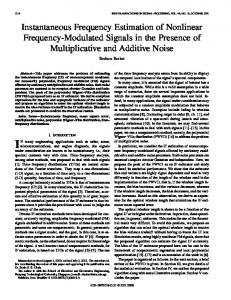
Fig. 1. Time-frequency analysis of a noisy signal. (a) Wigner distribution with N = 16: (b) Wigner distribution with N = 256: (c) Estimated instantaneous frequency using the Wigner distribution with N = 8: (d) Estimated instantaneous frequency using the Wigner distribution with N = 256: (e) Wigner distribution with adaptive window width. (f) Adaptive window width as function of time. (g) Estimated instantaneous frequency using the Wigner distribution with the adaptive window width. (h) Absolute mean error as a function of the window width; line represents the mean absolute error value for the adaptive window width.
the lower bound denoted Analogous conditions and These conditions may be written as hold for
(11)
(12) Having in mind (9), it can be verified that
According to (5) and (10) this results in (13)
´ AND KATKOVNIK: INSTANTANEOUS FREQUENCY ESTIMATION STANKOVIC
227
is the smallest satisfying the first inequality in (12). from (13) the second inequality in (12) is satisfied for With
The estimation of signal and noise parameters and can be done using The where variance is estimated by
(14) with
For the WD, which is considered as an example, we have It gives and The lower bound for is determined by the condition that Thus, we see that the conditions (11), along with can be easily satisfied. Taking, the condition that we for example, a value of such that get that all conditions of the statement are satisfied, as well for the Gaussian distribution of the error as, With (13) and (14) being satisfied we have for and for with This completes the proof. probability A search of the optimal window width over a finite set is a simplified optimization, because consists of a relatively small number of elements. However, the discrete set of inevitably leads to a suboptimal window width value due to the discretization of since, in general, the optimal window does not belong to i.e., it cannot be written as width It is important to note that this discretization of effect would also exist even if we knew in advance all of the parameters required for the optimal window width calculation, and decided to use radix-2 FFT algorithms in the realization. and then use the nearest one of the Then we should find Thus, the discretization of effect is present in any form case. It always results in worse values of the MSE, but that is the price of the algorithm efficiency. Fortunately, this loss of the accuracy is not significant in many cases, because the MSE (3) has a stationary point for the optimal window width (and the MSE varies very slowly for the window width values close to III. EXAMPLE The discrete pseudo-WD with the rectangular lag-window is calculated using the standard FFT routines, as In the example, we assumed a signal of the form with a given IF, and the phase The signal amplitude was and [dB], The time interval considered was with A set of window widths corresponding to the following number of signal samples is considered. The WD is calculated from the smallest toward the wider window widths. All distributions are interpolated up to the largest number of samples in order to have the same number of frequency samples and to reduce the quantization error whose variance and may also be included as a part of is total estimation variance. The IF is estimated using (2). According to the estimated IF and the segments (10) are when defined with, for example,
and being the real and imaginary part of It is assumed that is large, as well as is small. For this estimation, we used signal oversampled by factor of is determined as the four. The adaptive window width when width corresponding to the largest (8) is still satisfied, i.e., when still
The WD’s with constant window widths and are presented in Fig. 1(a) and (b), respectively. The IF estimates using the WD’s with constant window widths and are given in Fig. 1(c) and (d). Fig. 1(e) shows the WD with adaptive window width whose values determined by the algorithm are given in Fig. 1(f). We can see that when the IF variations are small, the algorithm uses the widest window width in order to reduce the variance. where the IF variations are large, Around the point the windows with smaller widths are used. The IF estimate with adaptive window width is presented in Fig. 1(g). Mean absolute error, normalized to the discretization step, is shown in Fig. 1(h) for each considered window width. Line represents its value for the adaptive window width. Additional examples and realization details may be found in [6]. We can conclude that the adaptive window width estimation, using the algorithm derived in this letter, has lower error than the best constant-window case, which, by the way, is also not known in advance. ACKNOWLEDGMENT The authors are very thankful to the Associate Editor and reviewers for remarks that helped in preparing the final version of this letter. REFERENCES [1] M. G. Amin, “Minimum variance time-frequency distribution kernels for signals in additive noise,” IEEE Trans. Signal Processing, vol. 44, pp. 2352–2356, Sept. 1996. [2] B. Boashash, “Estimating and interpreting the instantaneous frequency of a signal-Part 1: Fundamentals,” Proc. IEEE, vol. 80, pp. 519–538, Apr. 1992. [3] L. Cohen and C. Lee, “Instantaneous bandwidth,” in Time-Frequency Signal Analysis, B. Boashash, Ed. Australia: Longman Cheshire, 1992. [4] A. Goldenshluger and A. Nemirovski, “On spatial adaptive estimation of nonparametric regression,” Res. Rep., 5/94, Technion—Israel Inst. Technol., Haifa, Nov. 1995. [5] V. Katkovnik, “Adaptive local polynomial periodogram for time-varying frequency estimation,” in Proc. IEEE-SP IS-TFTSA, Paris, France, June 1996, pp. 329–332. [6] V. Katkovnik and LJ. Stankovi´c, “Instantaneous frequency estimation using the Wigner distribution with varying and data-driven window length,” IEEE Trans. Signal Processing, vol. 46, pp. 2315–2325, Sept. 1998. [7] P. Rao and F. J. Taylor, “Estimation of the instantaneous frequency using the discrete Wigner distribution,” Electron. Lett., vol. 26, pp. 246–248, 1990. [8] LJ.Stankovi´c, S. Stankovi´c, “On the Wigner distribution of discrete-time noisy signals with application to the study of quantization effects,” IEEE Trans. Signal Processing, vol. 42, pp. 1863–1867, July 1994.