Nov 21, 2018 - a ConvNet with only 1x1 convolutions while spatial convolutions ... contain depth-wise, group, dilated, and factorized convolutions. Not all of ...
Synetgy: Algorithm-hardware Co-design for ConvNet Accelerators on Embedded FPGAs Yifan Yang1,2,∗ , Qijing Huang1 , Bichen Wu1 , Tianjun Zhang1 , Liang Ma3 , Giulio Gambardella4 , Michaela Blott4 , Luciano Lavagno3 , Kees Vissers4 , John Wawrzynek1 , Kurt Keutzer1
arXiv:1811.08634v1 [cs.CV] 21 Nov 2018
1 UC
Berkeley; 2 Tsinghua University; 3 Politecnico di Torino; 4 Xilinx Research Labs {yifan-yang,qijing.huang,bichen,tianjunz,johnw,keutzer}@berkeley.edu; {luciano.lavagno,liang-ma}@polito.it;{guiliog,mblott,keesv}@xilinx.com
ABSTRACT Using FPGAs to accelerate ConvNets has attracted significant attention in recent years. However, FPGA accelerator design has not leveraged the latest progress of ConvNets. As a result, the key application characteristics such as frames-per-second (FPS) are ignored in favor of simply counting GOPs, and results on accuracy, which is critical to application success, are often not even reported. In this work, we adopt an algorithm-hardware co-design approach to develop a ConvNet accelerator called Synetgy and a novel ConvNet model called DiracNet. Both the accelerator and ConvNet are tailored to FPGA requirements. DiractNet, as the name suggests, is a ConvNet with only 1x1 convolutions while spatial convolutions are replaced by more efficient shift operations. DiracNet achieves competitive accuracy on ImageNet (89.0% top-5), but with 48x fewer parameters and 65x fewer OPs than VGG16. We further quantize DiracNet’s weights to 1-bit and activations to 4-bits, with less than 1% accuracy loss. These quantizations exploit well the nature of FPGA hardware. In short, DiracNet’s small model size, low computational OP count, ultra-low precision and simplified operators allow us to co-design a highly customized computing unit for an FPGA. We implement the computing units for DiracNet on an Ultra96 SoC system through high-level synthesis. The implementation only took 2 people 1 month to complete. Our accelerator’s final top-5 accuracy of 88.3% on ImageNet, is higher than all the previously reported embedded FPGA accelerators. In addition, the accelerator reaches an inference speed of 72.8 FPS on the ImageNet classification task, surpassing prior works with similar accuracy by at least 12.8x.
1
INTRODUCTION
ConvNets power state-of-the-art solutions on a wide range of computer vision tasks. However, the high computational complexity of ConvNets hinders their deployment on embedded and mobile devices, where computational resources are limited. Using FPGAs to accelerate ConvNets has attracted significant research attention in recent years. FPGAs excels at low-precision computation, and their adaptability to new algorithms lends themselves to supporting rapidly changing ConvNet models. Despite recent efforts to use FPGAs to accelerate ConvNets, as [1] points out, there still exists a wide gap between accelerator architecture design and ConvNet model design. The computer vision community has been primarily focusing on improving the accuracy of ConvNets on target benchmarks with only secondary attention to the computational cost of ConvNets. As a consequence, *Work done while interning at UC Berkeley.
recent ConvNets have been trending toward more layers [2], more complex structures [3, 4], and more complicated operations [5]. On the other hand, FPGA accelerator design has not leveraged the latest progress of ConvNets. Many FPGA designs still focus on networks trained on CIFAR10 [6], a small dataset consisting of 32x32 thumbnail images. Such dataset is usually used for experimental purposes and is too small to have practical value. More recent designs aim to accelerate inefficient ConvNets such as AlexNet [7] or VGG16 [8], both of which have fallen out of use in the state-ofthe-art computer vision applications. In addition, we observe that in many previous designs, key application characteristics such as frames-per-second (FPS) are ignored in favor of simply counting GOPs, and accuracy, which is critical to applications, is often not even reported. Specifically, we see a gap between ConvNet architectures and accelerator design in the following areas: Inefficient ConvNet models: Many FPGA accelerators still target older, inefficient models such as AlexNet and VGG16, which require orders-of-magnitude greater storage and computational resources than newer, efficient models that achieve the same accuracy. With an inefficient model, an accelerator with high throughput in terms of GOPs can actually have low inference speed in terms of FPS, where FPS is the more essential metric of efficiency. To achieve AlexNet-level accuracy, SqueezeNet [9] is 50x smaller than AlexNet; SqueezeNext [10] is 112x smaller; ShiftNet-C [11], with 1.6% higher accuracy, is 77x smaller. However, not many designs target those efficient models. Additionally, techniques for accelerating older models may not generalize to newer ConvNets. ConvNet structures: Most ConvNets are structured solely for better accuracy. Some ConvNets are structured for optimal GPU efficiency, but few, if any, are designed for optimal FPGA efficiency. For example, the commonly used additive skip connection [12] alleviates the difficulty of training deep ConvNets and significantly boosts accuracy. Despite its mathematical simplicity, the additive skip connection is difficult to efficiently implement on FPGAs. Additive skip connections involve adding the output data from a previous layer to the current layer, which requires either using on-chip memory to buffer the previous layer’s output or fetching the output from off-chip memory. Both options are inefficient on FPGAs. ConvNet operators: ConvNet models contain many different types of operators. Commonly used operators include 1x1, 3x3, 5x5 convolutions, 3x3 max pooling, etc. More recent models also contain depth-wise, group, dilated, and factorized convolutions. Not all of these operators can be efficiently implemented on FPGAs. If a ConvNet contains many different types of operators, one must either allocate more dedicated compute units or make the
2 BACKGROUND 2.1 Efficient ConvNet Models
compute unit more general. Either solution can potentially lead to high resource requirement, limited parallelism, and more complicated control flow. Also, hardware development will require more engineering effort. Quantization: ConvNet quantization has been widely used to convert weights and activations from floating point to low-precision numbers to reduce the computational cost. However, many of the previous methods are not practically useful for FPGAs due to the following problems: 1) Quantization can lead to serious accuracy loss, especially if the network is quantized to ultra low precision numbers (less than 4 bits). Unfortunately, carefully reporting accuracy has not been the norm in the FPGA community. This is not tolerable for many computer vision applications. 2) Many of the previously presented quantization methods are only effective on large ConvNet models such as VGG16, AlexNet, ResNet, etc. Since those models are known to be redundant, quantizing those to low-precisions is much easier. We are not aware of any previous work tested on efficient models such as MobileNet or ShuffleNet. 3) Many methods do not quantize weights and activations directly to fixed point numbers. Usually, quantized weights and activations are represented by fixed-point numbers multiplied by some shared floating point coefficients. Such representation requires more complicated computation than purely fixed-point operations, and are therefore more expensive. In this work, we adopt an algorithm-hardware co-design approach to develop a ConvNet accelerator called Synetgy and a novel ConvNet model called DiracNet. Both the accelerator and the ConvNet are tailored to FPGAs and are optimized for ImageNet accuracy and inference speed (in terms of FPS). Our co-design approach produces a novel ConvNet architecture DiracNet that is based on ShuffleNetV2 [13], one of the state-of-the-art efficient models with small model size, low FLOP counts, hardware friendly skip connections, and competitive accuracy. We optimize the network by replacing all 3x3 convolutions with shift operations [11] and 1x1 convolution, enabling us to implement a compute unit customized for 1x1 convolutions for better efficiency. The name “DiracNet” comes from the fact that the network only convolves input feature maps with 1x1 kernels. Such kernel functions can be seen as discrete 2D Dirac Delta functions. We further quantize the network to have 1-bit (binary) weights and 4-bit activations, exploiting the strengths of FPGAs, with only a less than 1% accuracy drop. To our knowledge, our work is the first to report such high compression on efficient models. In short, DiracNet’s small model size, low operation count, ultra-low precision and simplified operators allow us to co-design a highly customized and efficient FPGA accelerator. Furthermore, the implementation only took two people working for one month using HLS. We trained DiracNet on ImageNet, implemented it on our accelerator architecture and deployed on a low-cost FPGA board (Ultra96). Our inference speed reaches 72.8 FPS, surpassing previous works with similar accuracy by at least 12.8x. The DiracNet on our accelerator architecture also achieves 88.3% top-5 classification accuracy – the highest among all the previously reported embedded FPGA accelerators.
For the task of image classification, improving accuracy on the ImageNet [14] dataset has been the primary focus of the computer vision community. For applications that are sensitive to accuracy, even a 1% improvement in accuracy on ImageNet is worth doubling or tripling model complexity. As a concrete example, ResNet152 [12] achieves 1.36% higher ImageNet accuracy than ResNet50 at the cost of 3x more layers. In recent years, efficient ConvNet models have begun to receive more research attention. SqueezeNet is one of the early models focusing on reducing the parameter size. While SqueezeNet is designed for image classification, later models, including SqueezeDet [15] and SqueezeSeg [16, 17], extend the scope to object detection and point-cloud segmentation. More recent models such as MobileNet [18, 19] and ShuffleNet [13, 20] further reduce model complexity. However, without a target computing platform in mind, most models designed for “efficiency” can only target intermediate proxies to efficiency, such as parameter size or FLOP count, instead of focusing on more salient efficiency metrics, such as speed and energy. Recent works also try to bring in hardware insight to improve the actual efficiency. SqueezeNext[10] uses a hardware simulator to adjust the macro-architecture of the network for better efficiency. ShiftNet[11] proposes a hardware-friendly shift operator to replace expensive spatial convolutions. AddressNet[21] designed three shift-based primitives to accelerate GPU inference.
2.2
ConvNet Quantization
ConvNet quantization aims to convert full-precision weights and activations of a network to low-precision representations to reduce the computation and storage cost. Early works [22, 23] mainly focus on quantizing weights while still using full-precision activations. Later works [24–27] quantize both weights and activations. Many previous works [23–25] see serious accuracy loss if the network is quantized to ultra low precisions. Normally, an accuracy loss of more than 1% is already considered significant. Also, in many works [23, 26], quantized weights or activations are represented by lowprecision numbers multiplied with some floating point coefficients. This can bring several challenges to hardware implementation. Last, but not least, most of the previous works report quantization results on inefficient models such as VGG, AlexNet, and ResNet. Given that those models are redundant, quantizing them to lower precisions is much easier. We have not yet seen any work which successfully applies quantization to efficient models.
2.3
Hardware Designs
Most existing ConvNet hardware research has focused on improving the performance of either standalone 3 × 3 convolution layers or a full-fledged, large ConvNet on large FPGA devices. [28] quantitatively studies the computation throughput and memory bandwidth requirement for ConvNets. [29] and [30] present their own optimization for ConvNets based on analytical performance models. They achieve high throughput on VGG16 using their proposed design methodology with OpenCL. [31] design convolution in frequency domain to reduce the compute intensity of the ConvNet. They demonstrate good power performance results on VGG16, 2
AlexNet, and GoogLeNet. [32] implements a ternary neural network on high-end Intel FPGAs and achieves higher performance/Watt than Titan X GPU. Most of the works mentioned above and others [33][34][35], target inefficient ConvNets on middle to high-end FPGA devices. For compact ConvNets, [36] demonstrates a binary neural network(BNN) FPGA design that performs CIFAR10 classification at 21906 frames per second(FPS) with 283 µs latency on Xilinx ZC706 device. The BNN reports an accuracy of 80.1%. [37] [38] run the BNN on a smaller device ZC7020. Although all three works achieve promising frame rates, they have not implemented larger neural networks for the ImageNet classification. It should be noted that classification on CIFAR10 dataset is orders of magnitude simpler than ImageNet, since CIFAR10 contains 100x fewer classes, 26x fewer images, and 49x fewer pixels in each image. Networks trained on CIFAR10 dataset also have way smaller complexity compared to those trained on ImageNet. In comparison, networks for ImageNet classification are closer to real-world applicability. [39] first attempted to deploy VGG-16 for ImageNet classification on embedded device zc7020 and achieved a frame rate of 4.45 fps. Later [40] improved the frame rate to 5.7 fps. However, their frame rate was relatively low for real-time image classification tasks. [41] [42] [39] have achieve high frame rate on smaller devices, however, the accuracy of their network is not on par with [40] for ImageNet classification.
3
Channel Split
1x1 Conv BN ReLU
3x3 DWConv Stride=2
3x3 DWConv BN
1x1 Conv
1x1 Conv BN ReLU
BN ReLU BN
1x1 Conv
BN ReLU
Concat & Shuffle
BN ReLU
Concat & Shuffle
(a) ShuffleNetV2 blocks [13].
Channel Split 1x1 Conv 1x1 Conv ActQuant
2x2 Maxpool Stride=2
2x2 Maxpool Stride=2
Shift ActQuant
1x1 Conv
1x1 Conv
ActQuant Concat & Shuffle
CONVNET DESIGN
ActQuant
Shift
1x1 Conv
ActQuant Concat & Shuffle
(b) Our modified DiracNet blocks. We replace depthwise convolutions with shift operations. In the downsampling blocks, we use stride-2maxpooling and shift operations to replace stride-2-depthwise convolutions. We also double the filter number of the 1st 1x1 convolution on the non-skip branch in each module.
We discuss the ConvNet design in this section. An ideal ConvNet model for embedded FPGA acceleration should satisfy the following aspects: 1) The network should not contain too many parameters or FLOPs but still maintain a competitive accuracy. 2) The network structure should be hardware friendly to allow efficient scheduling. 3) The network’s operation set should be simplified for efficient FPGA implementation. 4) The network’s weights and activations should be quantized to low-precision fixed-point numbers without much accuracy loss.
3.1
1x1 Conv
3x3 DWConv Stride=2
Figure 1: ShuffleNetV2 blocks vs. DiracNet blocks.
We select ShuffleNetV2-1.0x not only because of its small model size and low FLOP count, but also because it uses concatenative skip connections instead of additive skip connections. Additive skip connection, as illustrated in Fig. 2(a), were first proposed in [12]. It effectively alleviates the difficulty of training deep neural networks and therefore improve accuracy. It is widely used in many ConvNet designs. However, additive skip connections are not efficient on FPGAs. As illustrated in Fig. 2(a), both the skip and the residual branches’ data need to be fetched on-chip to conduct the addition. Though addition does not cost too much computation, the data movement is expensive. Concatenative skip connections, as illustrated in Fig. 2(b), were first proposed in [3]. It has a similar positive impact to the network training and accuracy. With concatenative skip connections, data from skip branch is already in off-chip DRAMs. So we can concatenate the two branches simply by writing the residual branch data next to the skip branch data. This avoids the extra memory access in additive skip connections and alleviates the memory bandwidth pressure.
ShuffleNetV2
We select ShuffleNetV2-1.0x [13] as our starting point. ShuffleNetV2 is one of the state-of-the-art efficient models. It has a top-1 accuracy of 69.4% on ImageNet (2% lower than VGG16), but contains only 2.3M parameters (60x smaller than VGG16) and 146M FLOPs (109x smaller than VGG16). The block-level structure of ShuffleNetV2 is illustrated in Fig. 1(a). The input feature map of the block is first split into two parts along the channel dimension. The first branch of the network does nothing to the input data and directly feeds it to the output. The second branch performs a series of 1x1 convolutions, 3x3 depthwise convolutions and another 1x1 convolution to process the input. Outputs of two branches are then concatenated along the channel dimension. Channel shuffle [20] is then applied to exchange information between branches. In down-sampling blocks, depth-wise 3x3 convolutions with a stride of 2 are applied to both branches of the block to reduce the spatial resolution. 1x1 convolutions are used to double the channel size of input feature maps. These blocks are cascaded to build a deep ConvNet. We refer readers to [13] for the macro structure description of the ShuffleNetV2.
3.2
DiracNet
Based on ShuffleNetV2, we build DiractNet through the following modifications: 1) we replace all the 3x3 convolutions with shift and 1x1 convolutions; 2) we reduce the kernel size of max pooling from 3x3 to 2x2; 3) we modify the order of channel shuffle. 3
Skip branch
Fetch
Residual branch
+
Skip branch
Residual branch
Fetch
Write
Write
(a) Transpose based channel shuffle (a) Additive skip connection
(b) Concatenative skip connection
Figure 2: Additive skip connections vs. concatenative skip connections. Rectangles represent data tensors. (b) Our channel shuffle
We replace all the 3x3 convolutions and 3x3 depthwise convolutions with shift operations and 1x1 convolutions. The motivation is that smaller convolution kernel sizes require less reuse of the feature map, resulting in a simpler data movement schedule, control flow, and time constraint. As pointed out by [11], ConvNets rely on spatial convolutions (3x3 convolutions and 3x3 depth-wise convolutions) to aggregate spatial information from neighboring pixels to the center position. However, spatial convolutions can be replaced by a more efficient operator called shift. The shift operator aggregates spatial information by copying nearby pixels directly to the center position. This is equivalent to shifting one channel of feature map towards a certain direction. When we shift different channels in different directions, the output feature map’s channel will encode all the spatial information. A comparison between 3x3 convolution and shift is illustrated in Fig. 4. A module containing a shift and 1x1 convolution is illustrated in Fig. 5. For 3x3 depth-wise convolutions, we directly replace them with shift operations, as shown in Fig. 1(b). This direct replacement can lead to some accuracy loss. To mitigate this, we double the output filter number of the first 1x1 convolution on the non-skip branch from Fig. 1(b). Nominally, doubling the output channel size increases both FLOP count and parameter size by a factor of 2. However, getting rid of 3x3 convolutions allows us to design a computing unit customized for 1x1 convolutions with higher execution efficiency than a comparable unit for 3x3 depth-wise convolutions. In the downsample block, we directly replace the strided 3x3 depthwise convolutions with a stride-2 2x2 max pooling. Unlike [11], our shift operation only uses 4 cardinal directions (up, down, left, right) in addition to the identity mapping (no-shift). This simplifies our hardware implementation of the shift operation without hurting accuracy. The first stage of ShuffleNetV2 consists of a 3x3 convolution with a stride of 2 and filter number of 24. It is then followed by a 3x3 maxpooling with a stride of 2. We replace these two layers to a module consisting of a series of 1x1 convolution, 2x2 max pooling, and shift operations, as shown in Table. 1. Compared with the original 3x3 convolutions, our proposed module has slightly fewer parameters (612 vs 648) and slightly more FLOPs (9.0M vs 8.1M). After training the network, we find that this module gives better accuracy than the original 3x3 convolution module. With our new module, we can eliminate the remaining 3x3 convolutions from our network, enabling us to allocate more computational resources to 1x1 convolutions, and thereby increasing parallelism and throughput. In addition to replacing all 3x3 convolutions, we also reduce the max pooling kernel size from 3x3 to 2x2. By using the same
Figure 3: Transpose based shuffle (ShuffleNetV2) vs. our HW efficient shuffle (DiracNet)
pooling kernel size as the stride, we eliminate the need to buffer extra data on the pooling kernel boundaries, thereby achieving better efficiency. Our experiments also show that reducing the max pooling kernel size does not impact accuracy. We also modify the channel shuffle’s order to make it more hardware efficient. ShuffleNetV2 uses transpose operation to mix channels from two branches. This is illustrated in Fig. 3(a), where blue and red rectangles represent channels from different branches. The transpose based shuffling is not hardware friendly, since it breaks the contiguous data layout. Performing channel shuffle in this manner will require multiple passes of memory read and write. We propose a more efficient channel shuffle showed in Fig. 3(b). We perform a circular shift to the feature map along the channel dimension. We can have the same number of channels exchanged between two branches while preserving the contiguity of the feature map and minimizing the memory accesses. We name the modified ShuffleNetV2-1.0x model as DiracNet. The name comes from the fact that our network only contains 1x1 convolutions. With a kernel size of 1, the kernel functions can be seen as discrete 2D Diract Delta functions. DiracNet’s macro-structure is summarized in Table 1. Stage 2,3,4 consist of chained DiracNet blocks depicted in Fig. 1 with different feature map size, channel size and stride. We adopt the training recipe and hyperparameters described in [13]. We train DiracNet for 360 epoch with linear learning rate decay, the initial learning rate of 0.5, 1024 batch size and 4e-5 weight decay. A comparison between ShuffleNetV2-1.0x and our DiracNet is summarized in Table 2.
3.3
ConvNet Quantization
To further reduce the cost of DiracNet, we apply quantization to convert floating point weights and activations to low-precision integer values. For network weights, we follow DoReFA [25] to quantize full-precision weights as w k = 2Q k (
tanh(w) + 0.5) − 1. 2max(| tanh(w)|)
(1)
Here, w denotes the latent full-precision weight of the convolution kernel. Q k (·) is a function that quantizes its input in the range of [0, 1] to its nearest neighbor in { 2ki−1 |i = 0, · · · 2k −1 }. 4
Table 1: Macro-structure of DiracNet. Output size 224 224 112 112 112 56 56 28 28 14 14 7 7 7 1
Layer Image Conv1 Maxpool shift Conv2 Maxpool shift Stage 2 Stage 3 Stage 4 Conv5 GlobalPool FC
Kernel size
Stride
#Repeat
1 2 1 1 2 1 2 1 2 1 2 1 1
1 1 1 1 1 1 1 3 1 7 1 3 1 1 1
1 2 3 1 2 3
1 7
x l is the activation of layer-l. PACT (·) is a function that clips the activation x l to the range between [0, α l ]. α l is a layer-wise trainable upper bound, determined by the training of the network. It is observed that during training α l can sometimes become a negative value, which affects the correctness of the PACT [26] function. To ensure α l is always positive and to increase training stability, we use the absolute value of the trainable parameter α l rather than its original value. y l is the clipped activation from layer-l and it is further quantized to ykl , a k-bit activation tensor. Note that activations from the same layer share the same floating point coefficient α l , but activations from different layers can have different coefficients. This is problematic for the concatenative skip connection, since if the coefficients α l and α l −1 are different, we need to first cast ykl −1 and ykl from fixed-point to floating point, re-calculate a coefficient for the merged activation, and quantize it again to new fixed-point numbers. This process is very inefficient. In our experiment, we notice that most of the layers in the DiracNet have similar coefficients with values. Therefore, we rewrite equation (2) as � � y l = Q k y l / α l · |s |. (3)
Output channel 3 12
48 116 232 464 1024 1024 1000
Table 2: ShuffleNetV2-1.0x vs. DiracNet. MACs 146M 244M
ShuffleNetV2-1.0x DiracNet
#Params 2.3M 2.9M
Top-1 acc 69.4% 69.6%
Top-5 acc 89.0%
where s is a coefficient shared by the entire network. This step ensures that activations from different layers of the network are quantized and normalized to the same scale of [0, |s |]. As a result, we can concatenate activations from different layers directly without extra computation. Moreover, by using the same coefficient s across the entire network, the convolution can be computed completely via fixed-point operations. The coefficient s can be fixed before or leave it as trainable. A general rule is that we should let s have similar values of α l from different layers. Otherwise, if s/α l is either too small or too large, it can cause gradient vanishing or exploding problems in training, which leads to a worse accuracy of the network. In our network, we merge the PACT function and activation quantization into one module and name it ActQuant. The input to ActQuant is the output of 1x1 convolutions. Since the input and weight of the convolution are both quantized into fixed-point integers, the output is also integers. Then, ActQuant is implemented as a look-up-table whose parameters are determined during training and fixed during inference. We follow [27] to quantize the network progressively from fullprecision to the desired low-precision numbers. The process is illustrated in Fig 6, where x-axis denotes bit-width of weights and y-axis denotes the bit-width of activations. We start from the fullprecision network, train the network to convergence, and follow a path to progressively reduce the precision for weights or activations. At each point, we train the network for 30 epochs with step learning rate decay. Formally, we denote each point in the grid as a quantization configuration Cw,a (Nw ). Here w represents the bitwidth of weight. a is the bitwidth of activation. Nw is the network containing the quantized parameters. The starting configuration would be the full precision network C32,32 (N 32 ). Starting from this configuration, one can either go down to quantize the activation or go right to reduce the bitwidth of weight. More aggressive steps can be taken diagonally or even across several grids.
(b) Shift
(a) 3x3 convolution
1 Figure 4: 3x3 convolution vs. shift. In 3x3 convolutions, pixels in a 3x3 regions are aggregated to compute one output pixel at the center position. In the shift operation, a neighboring pixel is directly copied to the center position. Shift DF
DF
DF
DF
⨷
…
M
N
DF
…
M
M
1x1 conv
DF
…
…
…
N
Figure 5: Using shift and 1x1 convolutions to replace 3x3 convolutions. This figure is from [11]. We follow PACT [26] to quantize each layer’s activation as � � x l − x l − α l + α l l l , y = PACT x = (2) � � 2 l l l l y = Q k y / α · α . 5
Weight 32
16
8
4
3
2
1
8
control, which enables us to further improve the hardware efficiency. The compute of the fully-connected layer can be mapped onto our convolution unit. And the remaining average-pooling layer which is not supported on the FPGA is instead offloaded to the ARM processor on the SoC platform.
4
4.1
activation 16
Because the compute graph of our network for ImageNet classification cannot be fully spatially mapped onto an embedded FPGA, a layer-based accelerator architecture is chosen for the design. This is also commonly called a “double buffered” [44] approach. For layer-based accelerators, partial outputs are normally fed back to the DRAM between layers due to the limited on-chip memory. Such a design exposes ample opportunities for efficiently supporting the shift and shuffle operations by simply changing the address offset either during input fetch or output writeback. The shuffle operation comes with little cost in the hardware. This is very economical compared with the residual addition operation in popular nets such as ResNet. In ResNet, the residual addition performs element-wise addition of outputs from the previous layer and current layer. The addition incurs more on-chip compute resources and imposes more pressure on the memory system as it is bandwidth bound. In this section, we will discuss our alternative approach, using the shift and shuffle operations, in detail.
Ours
3
2-Stage [26] 2
Progressive [26]
1
Figure 6: Quantization Grid Table 3: Quantization result on DiracNet Top-1 Acc Top-5 Acc
full 69.6% 89.0%
w16a16 69.6% 89.0%
w8a8 69.7% 89.0%
w4a4 68.3% 88.2%
w2a4 68.4% 88.3%
w1a4 68.3% 88.3%
The two-stage and progressive optimization methods proposed in [27] can be represented as two paths in Fig. 6. In our work, we start from C32,32 (N 32 ). Then we use N 32 to initialize N 16 and obtain C16,16 (N 16 ). And we apply step lr decay fine tuning onto N 16 to recover the accuracy loss due to the quantization. After several epochs of�fine-tuning, we get the desired low �
4.2
The accelerator architecture
Fig. 7 shows the overall accelerator architecture design. Our accelerator, highlighted in light yellow, can be invoked by the CPU for computing one 1 × 1 Conv-Pooling-Shift-Shuffle subgraph at a time. The CPU provides supplementary support to the accelerator. Both the FPGA and the CPU are used to run the network.
′ with no accuracy loss. Followprecision configuration C16,16 N 16 ing the same procedures, we are able to first go diagonally in the quantization grid to C4,4 (N 4 ). It is observed that if the bitwidth of activations are further reduced, the network will suffer from a significant accuracy loss (larger than 1%). So we change our quantization direction and walk horizontally in the grid to only quantizing weight while retaining the activation bitwidth. Finally we are able to quantize the network to C1,4 (N 1 ) with less than 1% top-5 accuracy loss compared to its full precision counterpart. The quantization path is presented as the red curve in Fig. 6. We use a pretrained ResNet50 label-refinery [43] to boost the accuracy of the quantized model. Even with such radical quantization, our quantized model still preserves a very competitive top-5 accuracy of 88.3%. Most of the previous quantization works [25– 27] are only effective on large models such as VGG16, AlexNet or ResNet50. To the best of our knowledge, we are the first to quantize efficient models to such low-precisions. Our quantization result is summarized in Table 3.
1 x 1 Conv Units
Weights
HARDWARE DESIGN
... ...
Conversion
out_fmap_local_0
out_fmap_local_2
out_fmap_local_1
out_fmap_local_3
Shuffle CPU
...
in_fmap_local_1
...
DDR DRAM
in_fmap_local_0 ...
4
Hardware-friendly Shuffle and Shift
Shift
Pooling
Controller
Figure 7: Accelerator Architecture
As mentioned in section 3.2, we aggressively simplified ShuffleNetV2’s operator set. Our modified network is mainly composed of the following operators: • 1×1 convolution • 2×2 pooling • shift • shuffle and concatenation Our accelerator is tailored to only support the operators above. This allows us to design more specialized compute units with simpler
In our quantized ConvNet, weights are 1-bit, input and output activations are 4-bit, and the largest partial sum is 13-bit. The width of partial sum is determined by the input feature bit width and the largest channel size. Given that the largest channel size is 464, there are 24 × 464 possible outcomes from the convolution, which requires 13 bits to represent. 4.2.1 Convolution Unit. The notations used in this section are listed in Table 4. As shown in Fig. 8, given an input feature map 6
Table 4: Notations Notation WIDTH HEIGHT IC IC_VEC IC_TOTAL OC OC_TOTAL N
Type variable variable constant: 12 constant: 6 variable constant: 12 variable constant: 8
Description width of feature map height of feature map number of input channel buffered on chip parallelism on input channel dimension total input channel size parallelism on output channel dimension total output channel size parallelism on width dimension
of size W I DT H × H EIGHT × IC_TOT AL and a weight kernel of size IC_TOT AL × OC_TOT AL, the generated output feature map is of size W I DT H × H EIGHT × OC_TOT AL in 1×1 convolution. The 1×1 convolution is essentially a matrix-matrix multiplication.
IC
Input Feature Maps
Output Feature Maps _ OC
IC
...
HEIGHT
L TA TO
_T OT AL
OC_TOTAL
_T OT AL
HEIGHT
Weights
Figure 9: Pseudo Code for Kernel Compute Scheduling 1x1
WIDTH
WIDTH
unit for the input feature is OC, which is set to 12. The theoretical maximum bandwidth of 1 HP port is around 4.32GB/s (assuming 128 bits running at 300MHz with 0.9 efficiency), which means 4.32 × 2 billion input features can be loaded. The theoretical memory bound throughput should be 12 × 4.32 × 2 = 104GMACs = 208GOPs. For compute bound problems, the attainable throughput is dependent on the compute capability. In our case, it is N × IC_V EC ×OC × f req = 8 × 6 × 12 × 300MHz = 173GMACs = 346GOPs. Based on the analysis, the convolution unit will reach the bandwidth bound before it hits the computation roofline.
Figure 8: 1×1 Convolution Although [1] suggests a weight stationary dataflow for 1 × 1 convolution dominant ConvNets, we find it not applicable to our design as the bit width of weights is much smaller than the partial sums (1 bit vs 13 bits). Transferring the partial sums on and off-chip will incur more traffic on the memory bus. Therefore, we adopt the output stationary dataflow by retaining the partial sums in the local register file until an output feature is produced. Fig. 9 shows how we schedule the workload onto the accelerator. Note that the nested loops starting at line 23, 25, 26 are automatically unrolled and all the inner loop computes are finished in one cycle. We first block our inputs so N ×IC_V EC ×OC multiplications can be mapped onto the compute units at each cycle (Line 23∼28). In every cycle, N × IC_V EC input features are fetched from the local buffer. They are convolved with OC number of weights of size IC_V EC and produces N ×OC partial sums. We pipeline the execution along the input channel dimension, so it takes IC/IC_V EC cycles to finish one N × IC × OC 1/4bit multiplication. The partial sums are stored in the fully partitioned LUT RAMs, which can be simultaneously accessed in every cycle. The parameter IC_V EC and N were tuned for the area performance tradeoff. Increasing IC_V EC increases overall resource utilization but helps to reduce the total number of execution cycles. Increasing N increases the reuse of weights when IC_TOT AL is larger than IC, but also demands larger local buffers to store the partial sums. In our current design, we set N to 8 and IC_V EC to 6. Based on the roofline model[45], the attainable throughput is the compute-to-communication(CTC) ratio multiplied by the bandwidth when it is bandwidth bound. The CTC ratio of our compute
4.2.2 Double Buffers. We use double buffering [44] to overlap the memory accesses with the kernel computation. We have 2 buffers for input features and 4 buffers for output features. We refer to them as in_fmap_local_ and out_fmap_local_ respectively in the paper. The input features are carefully laid out contiguously in the DRAM so that the AXI4 burst mode can be inferred in HLS. The burst mode reduces the total number of memory requests and thus saves the accelerator cycles in DRAM memory accesses. Specifically, as shown in Fig. 10, we store IC input features linearly in memory and fetch X × N of them into the in_fmap_local_ at a time. We pack 32 input features into 128-bit wide vector for every memory read. In order to fill the on-chip in_fmap_local_, it will need to finish IC × N × X × 4/128 memory accesses. Each memory access typically takes tens of FPGA cycles. We set X = 4 to roughly match the computation time. The output features are fed back to the DRAM in a similar manner. Two more output buffers are added to support the 2x2 pooling operation. The detailed design of the pooling layer will be discussed in the following sections. 4.2.3 Conversion Unit. The high bitwidth to low bitwidth conversion is performed immediately after the kernel computation. It is a step function with 16 intervals that converts 13-bit partial sum to 7
Memory Layout
IC
IC
Addr
32 x IC
32 x (2 x IC - 1)
32 x (IC + 1)
...
4.3 HEIGHT
32 x (IC - 1)
...
WIDTH / 32
HEIGHT
32
32
0
IC_TOTAL / IC
Addr
1
weight, the FC layer’s computation is mapped in a bit serial like manner. The convolution unit processes each bit of the FC weight iteratively and bit shift is done by configuring the step function in the conversion unit.
...
L
IC
TA
O _T
Input Feature Maps
...
WIDTH
...
Memory Layout AL OT _T
IC
Weights
OC
IC
Addr
IC x OC
IC x (OC + 1)
IC x (OC - 1)
... IC x (2 x OC - 1)
... 1x1
OC_TOTAL / OC
...
1x1
0
IC_TOTAL / IC
OC
OC_TOTAL
IC
... Addr
Software
We use the ARM processor to control the layer-based accelerator and to do the auxiliary memory copy work for the shuffle operation. The accelerator is set as a memory mapped slave to the host on the systems bus. Its memory access to the DRAM goes through the HP port in order to achieve high bandwidth. For the execution of each subgraph, the processor sets up the new pointer address for the memory inputs and outputs and the control parameters. If the subgraph requires a shuffle operation at the end of execution, the processor will start copying the identical map branch concurrently with the accelerator’s execution. The accelerator runs under a full Linux system, which controls the memory-mapped accelerator through the UIO driver interface. The Xilinx python-based PYNQ APIs [46] are used for fast deployment of the host software code on the Ultra 96 board.
...
...
4.4
Experimental Results
We implement our deep learning accelerators on the Ultra96 development board with Xilinx Zynq UltraScale+ MPSoC targeted at embedded applications. Table 5 shows the overall resource utilization of our implementation. We are able to utilize 79% of the total LUTs on the FPGA, as the bit-level 1/4bit multiplications are mapped onto LUTs and the fully-partitioned local buffers are also mapped onto LUT RAMs. BRAMs are mainly used for implementing the FIFOs. DSPs are used for the address calculation for the AXI protocol. Our implementation runs at 299 MHz. Power measurements are obtained via a power monitor. We measured 5.3W with no workload running on the programming logic side and 5.5W max power on the Ultra96 power supply line when running our network.
Figure 10: Input Layout in DRAM 4-bit activation. The threshold values are different for each layer. The local threshold values are updated from DRAM before each kernel computation. In hardware, this unit is implemented by using 16 comparators. They are mapped onto a binary tree structure to reduce the circuit latency. 4.2.4 Pooling Unit. Recall that we have four out_fmap_local_ for output double buffering. The extra set of the buffers is used for supporting the 2 × 2 pooling layer as it needs information from the previous row. We set the size of the buffer so that it can hold a whole row of output features. The loop to perform the pooling operation is fully unrolled along the row dimension, so a row of output features can be generated in one cycle.
Table 5: Resource Usage LUT 55666 (78.9%)
4.2.5 Shift Unit. With out_fmap_local_, we are able to hold a whole row of an image. Shifting left or right can be done by shifting the row vector. For shifting up and down, the accelerator simply needs to calculate the writeback address with a correct offset. The shift operation would not be as easy to support in other architecture as it requires the information from non-local past outputs.
FF 53764 (38.1%)
BRAM 63 (28.9%)
DSP 19 (5.3%)
We compare our accelerator against previous work in Table 6. As explained before, ConvNets for ImageNet classification are usually orders of magnitude more complex than CIFAR10 classification. Therefore, we only compare accelerators targeting ConvNets for ImageNet classification with a reasonable accuracy. Our work focuses on achieving competitive accuracy while improving the actual inference speed in terms of frames per second. Our experiments show that we successfully achieve those two goals. From the table, we can make the following observations: 1) Our accelerator achieves the highest top-1 and top-5 accuracy on ImageNet. The only previous work that comes close to our accuracy is [40], but its frame rate is 12.8x slower than ours. 2) Considering accelerators whose top-1 accuracy is 60%, which is a loose constraint, our model achieves the fastest inference speed. 3) Without the accuracy constraint, the speed of [41, 42, 47] can go as fast as 864.7 frames per second. But
4.2.6 Shuffle Unit. Shuffle is implemented also by changing the address offset of output features during the writeback phase. Since the shuffle operation still requires us to concatenate the output from the previous DiracNet block to the current DiracNet block outputs, the CPU is used to copy the output from previous DiracNet unit to the shuffled address. The memory copy operation should be done concurrently with the computation of current DiracNet unit. 4.2.7 Fully Connected Unit. We don’t explicitly design a dedicated unit to compute FC layer. Instead, we map the compute of FC layer onto our existing hardware convolution unit. The feature map size is 1 for the FC layer. While the convolution unit only supports 1bit 8
Table 6: Performance Comparison of Synetgy and previous works. Platform FPS Top-1 Acc Top-5 Acc Precision
VGG-SVD[39] Zynq XC7Z045 4.5 64.64% 86.66% 16b
AlexNet[47] Stratix-V 864.7 42.90% 66.80% 16b
VGG16[48] Stratix-V 3.8 66.58% 87.48% 8-16b
VGG16 [40] Zynq 7Z020 5.7 67.72% 88.06% 8b
DoReFa[42] Zynq 7Z020 106.0 46.10% 73.10% 2b
FINN-R [41] Zynq ZU3EG 200.0 50.3% N/A 1-2b
Throughput (GOPs)
136.97
1963.96
117.80
123
410.22
400
Frequency(MHz) Power(W)
150 3.0
150 26.2
120 19.1
214 3.0
200 2.3
220 10.2
Table 7: Frame Rate on Different Batch Size Batch Size Frame Rate
1 41.5
2 54.0
4 63.4
8 69.2
10 70.6
Ours Zynq ZU3EG 72.8 68.33% 88.31% 1-4b 35.53 (Overall) 138 (1x1 Conv) 299 5.5
Table 8: Runtime latency for different functional parts of the whole system.
16 72.8
their accuracy is rather low. 4) Our accelerator throughput is currently limited by low hardware utilization. However, our accelerate still achieves competitive frame rate, demonstrating the efficacy of our co-design methodology. We see the opportunity of significant frame rate improvement through further hardware optimization, which we will explore in the future. The reported framerate is achieved with batch size set to 16. There is a fixed software overhead for invoking the poll-based hardware accelerator. The computation latency of the Dirac layer Block1 in Table9 is 0.32ms for batch 1. The latency for a single read on the accelerator control register is 0.40ms, which is greater than the actual compute time. In order to minimize this software overhead, we increase the batch size to schedule more computation running on the accelerator per invocation. The frame rates of implementations with different batch sizes are summarized in Table 7. We intentionally design the hardware to have no reuse across the batch dimension for a fair comparison to other implementations. We break down the runtime of the whole heterogeneous system by bypassing one component of the system and measuring the runtime. The result is shown in table 8. The whole system runs at 70.6 FPS on ImageNet classification at a batch size of 10, including both hardware PE execution and software execution of average pooling, and shuffle. We can clearly see from the table that all non-conv components impact the overall performance slightly. To further understand the efficiency of various operators (1x1 conv, 2x2 max pooling, shift, and shuffle) implemented on FPGA and CPU, we measure the runtime of the DiracNet blocks with different configurations. The result is summarized in table 9. We test 2 blocks with different input feature map and channel size. Note that the theoretical OPs of block1 and block2 is the same. As shown in the table, shift incurs almost no performance drop onto the hardware. This is because shift is simply done by recalculating the output memory address(up and down) or bit shift (left and right). These operations don’t introduce new pipeline stages or stalling the pipeline. Max pooling improves the runtime performance because it halves memory write done by the FPGA. As is observed in table 9, memory copy latency of shuffle is completely hidden on block2 but not on block1. This is because memory copy overhead is proportional to HEIGHT ∗ W IDT H ∗ OC_TOT AL. But total OPs H EIGHT ∗ W IDT H ∗ IC_TOT AL ∗ OC_TOT AL remains the same, which means that smaller feature map will need less time
Overall w/o sw avg pool w/o fc w/o PYNQ API call w/o sw shuffle hw only
runtime (ms) (batch=10) 141.7 137.4 140.5
frame rate 70.6 72.8 71.2
134.2
74.5
136.2 130.8
73.4 76.5
Table 9: Runtime analysis for the first and last DiracNet blocks in different operator configurations.
feature map size in&out channel conv only conv+pool conv+shift conv+shuffle overall
runtime(ms) (batch=10) Block1 Block2 28 7 116 464 3.206 2.922 3.185 2.913 3.312 2.899 3.791 2.914 3.819 2.808
for memory copy. The memory copy overhead can be alleviated possibly through bare metal mode. Furthermore, better memory layout design could also reduce potential memory copy time.
5
CONCLUSION AND FUTURE WORKS
In this paper, we adopt an algorithm-hardware co-design approach to develop a ConvNet accelerator called Synetgy and a novel ConvNet model called DiracNet. Based on ShuffleNetV2, we optimize the network’s operators by replacing all the 3x3 convolutions with shift operations and 1x1 convolutions. This allows us to build a compute unit exclusively customized for 1x1 convolutions for better efficiency. We quantize the network’s weights to binary and activations to 4-bit fixed-point numbers with less than 1% accuracy loss. These quantizations very well exploit the nature of FPGA hardware. As a result, DiracNet has a small parameter size, low computational OPs, hardware-friendly skip connections, ultra-low precision, and simplified operators. These features allow us to implement highly customized and efficient accelerators on FPGA. We implement the network on Ultra96 Soc systems. The implementation only took two people one month using HLS tools. Our accelerator achieves 9
a top-5 accuracy of 88.3% on ImageNet, the highest among all the previously published embedded FPGA accelerators. It also reaches an inference speed of 72.8 FPS, surpassing prior works with similar accuracy by at least 12.8x. While we see many more opportunities for further optimization, we believe this demonstrates the efficacy of our co-design methodology. For the future works, we will focus on further hardware optimization. For example, we can use a direct dataflow approach to add more layers to the accelerator to improve the compute-tocommunication ratio. Correspondingly, we will need to adjust the network such that the computation subgraphs are more symmetric.
[21] H. Zhong, X. Liu, Y. He, and Y. Ma. Shift-based Primitives for Efficient Convolutional Neural Networks. ArXiv e-prints, September 2018. [22] Song Han, Huizi Mao, and William J Dally. Deep compression: Compressing deep neural networks with pruning, trained quantization and huffman coding. arXiv preprint arXiv:1510.00149, 2015. [23] Chenzhuo Zhu, Song Han, Huizi Mao, and William J Dally. Trained ternary quantization. arXiv preprint arXiv:1612.01064, 2016. [24] Mohammad Rastegari, Vicente Ordonez, Joseph Redmon, and Ali Farhadi. Xnornet: Imagenet classification using binary convolutional neural networks. In European Conference on Computer Vision, pages 525–542. Springer, 2016. [25] Shuchang Zhou, Yuxin Wu, Zekun Ni, Xinyu Zhou, He Wen, and Yuheng Zou. Dorefa-net: Training low bitwidth convolutional neural networks with low bitwidth gradients. arXiv preprint arXiv:1606.06160, 2016. [26] Jungwook Choi, Zhuo Wang, Swagath Venkataramani, Pierce I-Jen Chuang, Vijayalakshmi Srinivasan, and Kailash Gopalakrishnan. Pact: Parameterized clipping activation for quantized neural networks. arXiv preprint arXiv:1805.06085, 2018. [27] B. Zhuang, C. Shen, M. Tan, L. Liu, and I. Reid. Towards Effective Low-bitwidth Convolutional Neural Networks. arXiv preprint arXiv:1711.00205, 2017. [28] Chen Zhang, Peng Li, Guangyu Sun, Yijin Guan, Bingjun Xiao, and Jason Cong. Optimizing fpga-based accelerator design for deep convolutional neural networks. In Proceedings of the 2015 ACM/SIGDA International Symposium on FieldProgrammable Gate Arrays, pages 161–170. ACM, 2015. [29] Jialiang Zhang and Jing Li. Improving the performance of opencl-based fpga accelerator for convolutional neural network. In Proceedings of the 2017 ACM/SIGDA International Symposium on Field-Programmable Gate Arrays, pages 25–34. ACM, 2017. [30] Yufei Ma, Yu Cao, Sarma Vrudhula, and Jae-sun Seo. Optimizing loop operation and dataflow in fpga acceleration of deep convolutional neural networks. In Proceedings of the 2017 ACM/SIGDA International Symposium on Field-Programmable Gate Arrays, pages 45–54. ACM, 2017. [31] Chi Zhang and Viktor Prasanna. Frequency domain acceleration of convolutional neural networks on cpu-fpga shared memory system. In Proceedings of the 2017 ACM/SIGDA International Symposium on Field-Programmable Gate Arrays, pages 35–44. ACM, 2017. [32] Eriko Nurvitadhi, Ganesh Venkatesh, Jaewoong Sim, Debbie Marr, Randy Huang, Jason Ong Gee Hock, Yeong Tat Liew, Krishnan Srivatsan, Duncan Moss, Suchit Subhaschandra, et al. Can fpgas beat gpus in accelerating next-generation deep neural networks? In Proceedings of the 2017 ACM/SIGDA International Symposium on Field-Programmable Gate Arrays, pages 5–14. ACM, 2017. [33] Huimin Li, Xitian Fan, Li Jiao, Wei Cao, Xuegong Zhou, and Lingli Wang. A high performance fpga-based accelerator for large-scale convolutional neural networks. In Field Programmable Logic and Applications (FPL), 2016 26th International Conference on, pages 1–9. IEEE, 2016. [34] Utku Aydonat, Shane O’Connell, Davor Capalija, Andrew C Ling, and Gordon R Chiu. An opencl deep learning accelerator on arria 10. In Proceedings of the 2017 ACM/SIGDA International Symposium on Field-Programmable Gate Arrays, pages 55–64. ACM, 2017. [35] Xuechao Wei, Cody Hao Yu, Peng Zhang, Youxiang Chen, Yuxin Wang, Han Hu, Yun Liang, and Jason Cong. Automated systolic array architecture synthesis for high throughput cnn inference on fpgas. In Proceedings of the 54th Annual Design Automation Conference 2017, page 29. ACM, 2017. [36] Yaman Umuroglu, Nicholas J Fraser, Giulio Gambardella, Michaela Blott, Philip Leong, Magnus Jahre, and Kees Vissers. Finn: A framework for fast, scalable binarized neural network inference. In Proceedings of the 2017 ACM/SIGDA International Symposium on Field-Programmable Gate Arrays, pages 65–74. ACM, 2017. [37] Ritchie Zhao, Weinan Song, Wentao Zhang, Tianwei Xing, Jeng-Hau Lin, Mani Srivastava, Rajesh Gupta, and Zhiru Zhang. Accelerating binarized convolutional neural networks with software-programmable fpgas. In Proceedings of the 2017 ACM/SIGDA International Symposium on Field-Programmable Gate Arrays, pages 15–24. ACM, 2017. [38] Hiroki Nakahara, Tomoya Fujii, and Shimpei Sato. A fully connected layer elimination for a binarizec convolutional neural network on an fpga. In Field Programmable Logic and Applications (FPL), 2017 27th International Conference on, pages 1–4. IEEE, 2017. [39] Jiantao Qiu, Jie Wang, Song Yao, Kaiyuan Guo, Boxun Li, Erjin Zhou, Jincheng Yu, Tianqi Tang, Ningyi Xu, Sen Song, et al. Going deeper with embedded fpga platform for convolutional neural network. In Proceedings of the 2016 ACM/SIGDA International Symposium on Field-Programmable Gate Arrays, pages 26–35. ACM, 2016. [40] Kaiyuan Guo, Song Han, Song Yao, Yu Wang, Yuan Xie, and Huazhong Yang. Software-hardware codesign for efficient neural network acceleration. IEEE Micro, 37(2):18–25, 2017. [41] Michaela Blott, Thomas Preusser, Nicholas Fraser, Giulio Gambardella, Kenneth O’Brien, and Yaman Umuroglu. Finn-r: An end-to-end deep-learning framework for fast exploration of quantized neural networks, 2018.
REFERENCES [1] Kiseok Kwon, Alon Amid, Amir Gholami, Bichen Wu, Krste Asanovic, and Kurt Keutzer. Co-design of deep neural nets and neural net accelerators for embedded vision applications. arXiv preprint arXiv:1804.10642, 2018. [2] Kaiming He, Xiangyu Zhang, Shaoqing Ren, and Jian Sun. Identity mappings in deep residual networks. In European conference on computer vision, pages 630–645. Springer, 2016. [3] Gao Huang, Zhuang Liu, Laurens Van Der Maaten, and Kilian Q Weinberger. Densely connected convolutional networks. In CVPR, volume 1, page 3, 2017. [4] Barret Zoph, Vijay Vasudevan, Jonathon Shlens, and Quoc V Le. Learning transferable architectures for scalable image recognition. arXiv preprint arXiv:1707.07012, 2(6), 2017. [5] Fisher Yu and Vladlen Koltun. Multi-scale context aggregation by dilated convolutions. arXiv preprint arXiv:1511.07122, 2015. [6] Alex Krizhevsky and Geoffrey Hinton. Learning multiple layers of features from tiny images. Technical report, Citeseer, 2009. [7] Alex Krizhevsky, Ilya Sutskever, and Geoffrey E Hinton. Imagenet classification with deep convolutional neural networks. In Advances in neural information processing systems, pages 1097–1105, 2012. [8] Karen Simonyan and Andrew Zisserman. Very deep convolutional networks for large-scale image recognition. arXiv preprint arXiv:1409.1556, 2014. [9] Forrest N Iandola, Song Han, Matthew W Moskewicz, Khalid Ashraf, William J Dally, and Kurt Keutzer. Squeezenet: Alexnet-level accuracy with 50x fewer parameters and< 0.5 mb model size. arXiv preprint arXiv:1602.07360, 2016. [10] Amir Gholami, Kiseok Kwon, Bichen Wu, Zizheng Tai, Xiangyu Yue, Peter Jin, Sicheng Zhao, and Kurt Keutzer. Squeezenext: Hardware-aware neural network design. arXiv preprint arXiv:1803.10615, 2018. [11] Bichen Wu, Alvin Wan, Xiangyu Yue, Peter Jin, Sicheng Zhao, Noah Golmant, Amir Gholaminejad, Joseph Gonzalez, and Kurt Keutzer. Shift: A zero flop, zero parameter alternative to spatial convolutions. arXiv preprint arXiv:1711.08141, 2017. [12] Kaiming He, Xiangyu Zhang, Shaoqing Ren, and Jian Sun. Deep residual learning for image recognition. In Proceedings of the IEEE conference on computer vision and pattern recognition, pages 770–778, 2016. [13] Ningning Ma, Xiangyu Zhang, Hai-Tao Zheng, and Jian Sun. Shufflenet v2: Practical guidelines for efficient cnn architecture design. arXiv preprint arXiv:1807.11164, 2018. [14] Jia Deng, Wei Dong, Richard Socher, Li-Jia Li, Kai Li, and Li Fei-Fei. Imagenet: A large-scale hierarchical image database. In Computer Vision and Pattern Recognition, 2009. CVPR 2009. IEEE Conference on, pages 248–255. Ieee, 2009. [15] Bichen Wu, Forrest N Iandola, Peter H Jin, and Kurt Keutzer. Squeezedet: Unified, small, low power fully convolutional neural networks for real-time object detection for autonomous driving. In CVPR Workshops, pages 446–454, 2017. [16] Bichen Wu, Alvin Wan, Xiangyu Yue, and Kurt Keutzer. Squeezeseg: Convolutional neural nets with recurrent crf for real-time road-object segmentation from 3d lidar point cloud. arXiv preprint arXiv:1710.07368, 2017. [17] Bichen Wu, Xuanyu Zhou, Sicheng Zhao, Xiangyu Yue, and Kurt Keutzer. Squeezesegv2: Improved model structure and unsupervised domain adaptation for roadobject segmentation from a lidar point cloud. arXiv preprint arXiv:1809.08495, 2018. [18] Andrew G Howard, Menglong Zhu, Bo Chen, Dmitry Kalenichenko, Weijun Wang, Tobias Weyand, Marco Andreetto, and Hartwig Adam. Mobilenets: Efficient convolutional neural networks for mobile vision applications. arXiv preprint arXiv:1704.04861, 2017. [19] Mark Sandler, Andrew Howard, Menglong Zhu, Andrey Zhmoginov, and LiangChieh Chen. Mobilenetv2: Inverted residuals and linear bottlenecks. In Proceedings of the IEEE Conference on Computer Vision and Pattern Recognition, pages 4510–4520, 2018. [20] X Zhang, X Zhou, M Lin, and J Sun. Shufflenet: An extremely efficient convolutional neural network for mobile devices. arxiv 2017. arXiv preprint arXiv:1707.01083. 10
[42] Li Jiao, Cheng Luo, Wei Cao, Xuegong Zhou, and Lingli Wang. Accelerating low bit-width convolutional neural networks with embedded fpga. In Field Programmable Logic and Applications (FPL), 2017 27th International Conference on, pages 1–4. IEEE, 2017. [43] Hessam Bagherinezhad, Maxwell Horton, Mohammad Rastegari, and Ali Farhadi. Label refinery: Improving imagenet classification through label progression. arXiv preprint arXiv:1805.02641, 2018. [44] Chen Zhang, Peng Li, Guangyu Sun, Yijin Guan, Bingjun Xiao, and Jason Cong. Optimizing fpga-based accelerator design for deep convolutional neural networks. In Proceedings of the 2015 ACM/SIGDA International Symposium on FieldProgrammable Gate Arrays, FPGA ’15, pages 161–170, New York, NY, USA, 2015. ACM. [45] Samuel Williams, Andrew Waterman, and David Patterson. Roofline: An insightful visual performance model for floating-point programs and multicore architectures. Communications of the Association for Computing Machinery, 2009. [46] Xilinx. PYNQ Introduction, 2018. https://pynq.readthedocs.io/en/v2.3/. [47] Shuang Liang, Shouyi Yin, Leibo Liu, Wayne Luk, and Shaojun Wei. Fp-bnn: Binarized neural network on fpga. Neurocomputing, 275:1072–1086, 2018. [48] Naveen Suda, Vikas Chandra, Ganesh Dasika, Abinash Mohanty, Yufei Ma, Sarma Vrudhula, Jae-sun Seo, and Yu Cao. Throughput-optimized opencl-based fpga accelerator for large-scale convolutional neural networks. In Proceedings of the 2016 ACM/SIGDA International Symposium on Field-Programmable Gate Arrays, pages 16–25. ACM, 2016.
11