Algorithm-Hardware Codesign of Fast Parallel Round ... - CiteSeerX

1

Algorithm-Hardware Codesign of Fast Parallel Round-Robin Arbiters S. Q. Zheng† and Mei Yang‡ †

Department of Computer Science

University of Texas at Dallas, Richardson, TX 75083-0688, USA ‡

Department of Electrical and Computer Engineering

University of Nevada, Las Vegas, NV 89154-4026, USA Email: † [email protected], ‡ [email protected]

Abstract—As a basic building block of a switch scheduler, a fast and fair arbiter is critical to the efficiency of the scheduler, which is the key to the performance of a high-speed switch or router. In this paper, we propose a parallel round-robin arbiter (PRRA) based on a simple binary search algorithm, which is specially designed for hardware implementation. We prove that our PRRA achieves round-robin fairness under all input patterns. We further propose an improved (IPRRA) design that reduces the timing of PRRA significantly. Simulation results with TSMC .18µm standard cell library show that PRRA and IPRRA can meet the timing requirement of a terabit 256 × 256 switch. Both PRRA and IPRRA are much faster and simpler than the programmable priority encoder (PPE), a well-known round-robin arbiter design. We also introduce an additional design which combines PRRA and IPRRA and provides tradeoffs in gate delay, wire delay, and circuit area. With the binary tree structure and high performance, our designs are scalable for large N and useful for implementing schedulers for high-speed switches and routers.

conflict-free connections between input ports and output ports. Noticeably, in high performance switches, it is commonly that cell arriving, scheduling and switching, and departing are operated in a pipelined way [5]. All cells arriving in the current cell slot will be considered for scheduling and switching in the next cell slot. As the switching speed of the switching fabric increasing rapidly, the speed of the scheduler is critical to the performance of a switch. Input ports

Output ports

0

0 I0

1

I1

I2

I3

I4

I5

I6

I7 O0

1

O1 O2 O3 O4 O5

Keywords: Arbitration, circuits and systems, matching, parallel processing, round-robin arbiter, switch scheduling.

O6 O7 7

7

I. I NTRODUCTION

Scheduler

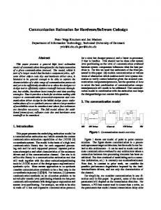
The growing demand for bandwidth fosters the need for terabit packet switches and routers. There are three major aspects in the design and implementation of a high-speed packet switch and router: (1) a cost-effective switching fabric that provides conflict-free paths between input ports and output ports; (2) a switch scheduling algorithm that chooses which packets to be sent from input ports to output ports; and (3) a fast mechanism that generates control signals for switching elements to set up confliction-free paths between inputs and outputs of the switching fabric. For a given switching fabric, a fast arbitration scheme can be used to implement (2) and (3). Hence, the design of a fast arbitration scheme is critical to the design of a high-speed packet switch or router [4], [15]. In this paper, we focus on the arbitration of a cell-based crossbar switch for unicast I/O connections. Consider an N ×N switch with N input ports I0 , I1 , · · · , IN −1 , and N output ports O0 , O1 , · · · ON −1 . Fig. 1(a) shows the block diagram of an 8 × 8 switch. Fig. 1(b) shows a crossbar switching fabric. To avoid head-of-line blocking [13], each input port maintains N virtual output queues (VOQs), each dedicated to holding cells destined for its associated output port. The task of the scheduling algorithm running in the scheduler is to decide a set of

(a)

(b)

Fig. 1. A 8 × 8 switch: (a) block diagram, and (b) crossbar switching fabric.

The cell scheduling problem for VOQ-based switches can be abstracted as a bipartite matching problem [16] on the bipartite graph composed of nodes of input ports and output ports and edges of connection requests from input ports to output ports. A maximum size matching is one with the maximum number of edges. A maximal size matching is one which cannot be included in any other matching. It has been proved that the size of a maximal size matching is at least half the size of a maximum size matching [12]. The most efficient maximum size matching algorithms [7], [21], running in O(N 2.5 ) time, are infeasible for high speed implementation and can cause unfairness [17]. Most practical scheduling algorithms proposed, such as PIM [1], iSLIP [16], DRRM [4], FIRM [18], SRR [10], and PPA [3], are iterative algorithms that approximate a maximum size matching by finding a maximal size matching. Most of these maximal size matching algorithms consist of multiple iterations, each composed of either three steps, Request-Grant-Accept (RGA), or two steps, Request-Grant (RG). All these algorithms can be implemented by the hard-

2

Grant/Request arbiters

Accept/Grant arbiters

0

0

1

1

first extracted from Req as Req thm = {Req i |i ≥ p}, where p is the selection starting point, using the thermometer vector generated from the thermometer encoder. Then the two priority encoders generate the grants for Req thm and Req respectively. The final grant vector Gnt is generated based on the two sets of grants Gnt thm and Gnt pre as follows: if there is any grant in Gnt thm, then Gnt = Gnt thm, otherwise, Gnt = Gnt pre. As one can see, both designs are too complicated for the simple round-robin scheme. p

N thermometer

Req_thm

N

priority encoder (thermo)

priority encoder Gnt_pre

Gnt_thm

N-1

Req log N

Decision registers

State memory and update logic

Requests from VOQs

ware scheduler architecture shown in Fig. 2 [16]. In such a scheduler, each input/output port is associated with an arbiter, and there are 2N such arbiters. Each arbiter is responsible for selecting one out of N requests. Output port arbiters operate in parallel to select their matched input ports respectively and input port arbiters operate in parallel to select their matched output ports respectively. Newly matched input/output pairs are added to previously matched pairs. This process continues until no more matched pairs can be found or a predetermined number of iterations is reached.

N

any_Gnt_thm

N

N-1

Fig. 2. Block diagram of a scheduler based on an RGA/RG maximal size matching algorithm. Gnt

Clearly, as the basic building block of the scheduler shown in Fig. 2, the design of a fast and fair arbiter is critical to the performance of the scheduler. Let Ts and Ta be the time for a cell slot and an arbitration cycle respectively, and let I be the number of iterations performed in a cell slot. In order for the scheduler to work properly, it must be 2Ta I ≤ Ts . If I is fixed, smaller Ta corresponds to smaller Ts . If Ts is fixed, smaller Ta means more iterations can be performed in each cell slot, which implies a larger matching can be found. An important issue in designing an arbiter is how to ensure fair service to all requesters. The most commonly used scheme for ensuring fairness is round-robin. In this scheme, all input ports are arranged as a directed loop. The input port that follows the input port being served in the current cell slot is assigned the highest priority in the next cell slot. The input port being served in the current slot is assigned the lowest priority in the next cell slot. The priorities of other input ports are determined by their positions in the loop starting from the input port that is being served. It is worthy to point out that the fairness in arbitration directly affects the fairness of the scheduler. A fair scheduler may not always yield a larger size matching, but it will improve the quality of service in terms of lower average cell delay. In [6], Gupta and McKeown surveyed previously wellknown round-robin arbiter designs, and proposed two new programmable priority encoder (PPE) designs, both having O(log N )-gate delay. Design 1 uses a (log N × N ) decoder, an N -bit ripple priority encoder, and a conventional N -bit priority encoder, each of which has O(log N )-gate delay. Design 2 improves Design 1 by using a log N × N thermometer decoder, and two N -bit priority encoders operating in parallel, as shown in Fig. 3. In this design, a subset of the requests Req thm is

any_Gnt

Fig. 3. Block diagram of the PPE design.

In [3], Chao et al. proposed the ping-pong arbiter (PPA), which features an O(log N )-level tree structure. Clearly, PPA has O(log N )-gate delay. Fig. 4 shows a 16-input ping-pong arbiter, featuring a 4-layer complete binary tree structure. Each node in the tree is a 2-input ping-pong arbiter (AR2). The basic function of an AR2 is favoring its two subtrees alternately if both subtrees have requests. By associating a 1-bit memory with each internal node of the tree, this arbiter implements the round-robin selection rule under the condition that all N requests are present in each cell slot. However, when there are less than N requests present, PPA can cause unfairness. For example, when N/2 + 1 input ports repeatedly request service in the pattern that one input port’s request is captured by one half of the tree and the remaining input ports’ requests are captured by the other half of the tree, this arbiter grants the one input port N/2 times more than each of the remaining N/2 input ports, resulting unfairness. In situations as such, PPA cannot provide round-robin fairness. One can see from Fig. 2 in [3] that the performance of scheduling algorithm based on PPA is worse than iSLIP and DRRM which are based on PPE. Using the same idea of “ping-pong” [3], another arbiter design, called switch arbiter (SA), was proposed in [19]. An SA is constructed by a tree structure composed of 4×4 SA nodes. An SA node consists of a D flip-flop, 4 priority encoders, a 4-bit ring counter, five 4-input OR gates, and four 2-input AND gates. SA is faster than PPA, but it is more complex in structure. As a PPA, the SA is not fair for nonuniformly distributed requests. In this paper, we show how to apply algorithm-hardware codesign to design simple and fast round-robin arbiters. We

3

group grant signal (layer 4)

group grant signal (layer 3)

group grant signal (layer 2)

external grant signal

input request signals

root AR2

internal AR2

Fig. 4. Block diagram of the PPA design.

present a parallel round-robin arbiter (PRRA) based on a simple binary search algorithm that is suitable for hardware implementation. PRRA is essentially a combinational circuit implementation of a binary tree structure. The arbitration process of PRRA consists of two traces, up-trace and down-trace. The up-trace is a subprocess of collecting the request and roundrobin priority information, and the down-trace is a subprocess of decision making based on the information collected in the up-trace. The PRRA design has O(log N )-gate delay and consumes O(N ) gates. We further present an improved (IPRRA) design that significantly reduces the timing of PRRA by overlapping up-traces and down-traces of all subtrees. Our simulation results with TSMC .18µm standard cell library show that PRRA and IPRRA can meet the timing requirement of a terabit 256 × 256 switch. Both PRRA and IPRRA are much faster and simpler than PPE. We also introduce an additional design which combines PRRA and IPRRA and provides tradeoffs in gate delay, wire delay, and circuit area. With the binary tree structure and high performance, our designs are scalable for large N and useful for implementing schedulers for high-speed switches and routers. The rest of the paper is organized as follows. Section II presents the design of PRRA and gives the analysis of its correctness and complexity. Section III generalizes PRRA and describes the improved PRRA (IPRRA) design. A general approach of finding tradeoffs among gate delay, wire delay, and circuit area is also presented. Section IV presents simulation results of PRRA and IPRRA and comparisons with PPE, PPA, and SA. Section V concludes the paper. II. D ESIGN OF PARALLEL ROUND -ROBIN A RBITER A. Problem Definition The function of request arbitration is defined as follows. Given binary inputs Ri and Hi , 0 ≤ i ≤ N − 1, compute binary outputs Gi , 0 ≤ i ≤ N − 1. Depending on the values of Hi ’s, we have two variations: HUA: Head Uniqueness Arbitration: At any arbitration time,

one and only one of Hi ’s can be in the 1-state. Assume that Hj = 1, Gi ’s are set as follows:   1 for i = (j + a) mod N, if there exists a = min{b | R(j+b) mod N = 1, 0 ≤ b ≤ N − 1}, Gi =  0 otherwise. (1) NHA: No Head Arbitration (NHA): If Hi = 0 for all 0 ≤ i ≤ N − 1, then   1 for i = a, if there exists a = min{j | Rj = 1, 0 ≤ j ≤ N − 1}, Gi =  0 otherwise. (2) HUA corresponds to round-robin priority, where Hi ’s are used as a circular pointer. NHA corresponds to linear-priority arbitration, for which all Hi = 0, implying that input 0 always has the highest priority. An arbiter is a hardware device that implements a given arbitration priority scheme. A round-robin arbiter implements HUA and the following additional functionality of updating Hi ’s after the operation specified in Eqn. (1): if Gi = 1 then Hi ← 0 and H(i+1) mod N ← 1. We aim at designing arbiters based on HUA, but we also consider NHA for the following two reasons: (i) HUA and NHA designs can be unified so that a single design is capable of handling both HUA and NHA; (ii) in our HUA designs, NHA can be used as an initiation step in the first arbitration cycle. B. Round-Robin Arbitration Search Algorithm Our goal is to design an optimal-time round-robin arbitration algorithm suitable for hardware implementation. Treating arbitration as a computation task, the problem of finding the desired input request among N possibilities requires Θ(log N ) time, regardless of the number of processing elements used as long as all basic processing elements are of interconnection degrees (i.e., the number of similar elements one element can be connected to) bounded by a constant. This is because the arbitration problem can be reduced to the problem of computing OR of N Boolean variables, which requires Ω(log N ) time [9]. The process of designing a special-purpose architecture (circuit or system) for a specific computational task is called algorithm-hardware codesign, which is a restricted form of widely known hardware-software codesign. The product of algorithm-hardware codesign is a high-performance hardware algorithm frequently invoked in a more complex computational environment. The methodology of algorithm-hardware codesign, and its generalization hardware-software codesign, is commonly adopted in designing embedded systems. For the algorithm-hardware codesign of round-robin arbiters, it is a natural choice to use a tree of bounded degree to characterize the arbitration processing structure, and apply parallel processing techniques to achieve the least possible processing time. In addition, the hardware implementation should be as simple as possible. Define a round-robin arbitration tree (RRA-tree) of size N as a (log N + 1)-level complete binary tree. Nodes are partitioned into levels. The node at level 0 is called the root node (r-node). Nodes at level 1 to level log N − 1 are called internal nodes (i-nodes). Nodes at level log N are called leaf nodes

4

r-node

11

11

i-nodes

01

11

00

01

01

0

1

2

3

l-nodes

Fig. 5. An RRA-tree for R0 R1 R2 R3 = 1011 and H0 H1 H2 H3 = 1000

S1 0

S0 0

0

1

1

0

1

1

States There is no Hk = 1 in the subtree rooted at u and the number of Ri = 1 in this subtree is 0 There is no Hk = 1 in the subtree rooted at u, and the number of Ri = 1 in this subtree is > 0. Hk = 1 is in the subtree rooted at u and the number of Ri = 1 such that i ≥ k in this subtree is 0. Hk = 1 is in the subtree rooted at u and the number of Ri = 1 such that i ≥ k in this subtree is > 0. TABLE I

S1

AND

S0

l- NODES OF A ( SUB ) TREE ROOTED AT AN i- NODE OR THE r- NODE .

USED TO CODE THE STATE OF

(l-nodes). The l-nodes of an RRA-tree are labeled from 0 to N − 1 from left to right such that Ri and Hi are associated with l-node i. Fig. 5 shows the structure of an RRA-tree of size 4. Following the binary tree structure, larger size RRA-trees can be constructed from smaller size RRA-trees recursively. The state of an RRA-tree is defined by Ri ’s and Hi ’s associated with its l-nodes. Let u be a node in an RRA-tree. We use two bits S 1 and S 0 to code the state of l-nodes in the subtree rooted at u as in Table I. Since the RRA-tree is recursively defined, its state is also recursively defined. For an l-node i, S 1 = Hi and S 0 = Ri . We associate the state of a (sub)tree T with its root node u, and we use the state of node u to refer to the state of T . In Fig. 5, the state of each node is given within the circle representing the node.

Now we present a simple binary search algorithm, named RRA-SEARCH, for finding the desired input request in an RRAtree, assuming that S 1 S 0 is available for every node in the tree. This algorithm is the basis of our round-robin arbiter designs, which will be given shortly. Let v and w be the left and right child of u respectively. We use S 1 S 0 (u), SL1 SL0 (u), and 1 0 SR SR (u) to denote the state of u, v, and w respectively. When node u is clear from the context, we omit u and use S 1 S 0 , 1 0 SL1 SL0 , and SR SR instead. Starting from the r-node, algorithm RRA-SEARCH recursively makes a decision of selecting the left subtree or right subtree, depending on the values of SL1 SL0 (u) 1 0 and SR SR (u) of the current node u until an l-node is reached. Table II gives the actions for all cases, where “left” or “right” indicates selecting the left or right substree of u respectively,

1 SL

0 SL

1 SR

0 SR

0 0 0 0 0 0 0 0 1 1 1 1 1 1 1 1

0 0 0 0 1 1 1 1 0 0 0 0 1 1 1 1

0 0 1 1 0 0 1 1 0 0 1 1 0 0 1 1

0 1 0 1 0 1 0 1 0 1 0 1 0 1 0 1

Action HUA NHA r-node i-node r-node i-node −− −− right right −− right right right right right −− −− right right −− −− −− left left left −− left left left left left −− −− right right −− −− left left −− −− right right −− −− −− −− −− −− −− −− −− −− left left −− −− left left −− −− −− −− −− −− −− −− −− −− TABLE II

S EARCH ACTION TO BE TAKEN AT A NON - LEAF NODE u.

1 0 SR and and “−−” indicates that the combination of SL1 SL0 SR the type of node u is impossible by the definition of S 1 S 0 coding under HUA or NHA. Impossible cases are included in the table for completeness even though they will not be encountered. Our algorithm RRA-SEARCH, which can be applied to HUA and NHA using corresponding columns in Table II, is as follows:

Algorithm RRA-SEARCH Input: An RRA-tree with state information available in every node. Output: The desired l-node if at least one l-node having non-zero request. begin Search the action in the column “r-node” of Table II using 1 S 0 S 1 S 0 of the r-node. SL L R R if the corresponding action is “left” then u ← left child of r; else u ← right child of r. while u is not an l-node do 1 S 0 S 1 S 0 of u as index to search the action in the Use SL L R R column “i-node” of Table II. if the corresponding action is “left” then u ← left child of u; else u ← right child of u. end-while if S 1 S 0 = ×0 for u then output “no desired request”; else output u. end

C. Correctness of RRA-SEARCH In this subsection, we prove the correctness of RRA-SEARCH algorithm when it is applied to HUA and NHA. Theorem 1: RRA-SEARCH algorithm is correct when it is applied to NHA. Proof: Since none of Hi ’s is 1, S 1 = 0 for every node of RRA1 0 1 0 tree. Thus, SL1 SL0 SR SR 6= 1 × ×× and SL1 SL0 SR SR 6= × × 1× 1 . The entries in the columns of r-node and i-node of Table II under NHA marked “−−” correspond to these impossible cases. 1 In the rest of this paper, symbol × is used to indicate a “don’t care” condition.

5

The only legal values of S 1 S 0 are 00 and 01. According to the definition of S 1 S 0 , S 1 S 0 = 00 and S 1 S 0 = 01 are recursively defined as shown in Fig. 6. By Table II, the actions taken from the r-node to an l-node by RRA-SEARCH can be modeled by a finite-state automata, with its states directly corresponding to the states of nodes in RRA-trees and its transition diagram shown in Fig. 7.

RRA-trees and its transition diagram shown in Fig. 9. In this figure, a double-circle represents the starting state. All states can be ending states. 10

01 00

01

10

10

10

00

01

00

00

10

01 11

00

10

0✕

00

11

11

01

Fig. 6. Recursive definition of S 1 S 0 = 00 and S 1 S 0 = 01.

0✕

11

0✕

11

10

01

Fig. 8. Recursive definition of S 1 S 0 = 10 and S 1 S 0 = 11.

0000/right

010✕ /left 01

00

(a)

010 ✕ /left

1000/left

0001/right

(b)

10

01

0010/right

0001/right

(a)

Fig. 7. State diagram describing RRA-SEARCH for NHA: (a) S 1 S 0 = 00 for the r-node; (b) S 1 S 0 = 00 for the r-node.

In Fig. 7, the value of S 1 S 0 is used to label the state of a 1 0 1 0 node, and SL1 SL0 SR SR /left (resp. SL1 SL0 SR SR /right) indicates RRA-SEARCH continues the search by selecting the left (resp. 1 0 right) subtree based on the values of SL1 SL0 SR SR of the current node. For a particular state S 1 S 0 of the r-node, the only state is the starting and ending state, and the state transitions follow the transition arcs. Suppose the state of the r-node is S 1 S 0 = 01, 1 0 if SL1 SL0 SR SR = 010× for the r-node, RRA-SEARCH selects the left branch of the RRA-tree, and the state of its left child is 1 0 also 01; if SL1 SL0 SR SR = 0001 for the r-node, RRA-SEARCH selects the right branch of the RRA-tree and the state of its right child is also 01. As shown in Fig. 7, the state repeats until it reaches an l-node with state S 1 S 0 = 01. From Table II, this lnode must hold the first non-zero request, which is the desired request. If the state of the r-node is 00, the selection action can be arbitrary since there is no desired request and any grant signal is meaningless. For simplicity, RRA-SEARCH selects the right branch. An input which currently has no request can simply ignore the received grant signal. Therefore, we conclude that RRA-SEARCH algorithm is correct for NHA. Theorem 2: RRA-SEARCH algorithm is correct when it is applied to HUA. Proof: For HUA, since one and exactly one of Hi ’s is 1, 1 0 SL1 SL0 SR SR = 1 × 1× is not possible. Also, for the r-node, 1 0 1 0 S S = 00 and SL1 SL0 SR SR = 0 × 0× are not possible. The entries in the columns of r-node and i-node of Table II under HUA marked “−−” correspond to these impossible cases. The only legal states for the r-node are 10 and 11. According to the definition of S 1 S 0 , S 1 S 0 = 10 and S 1 S 0 = 11 are recursively defined as shown in Fig. 8, which utilize the definitions of state 00 and 01 shown in Fig. 8 to complete the definition. By Table II, the actions taken from the r-node to an l-node by RRA-SEARCH can be modeled by a finite-state automata, with its states directly corresponding to the states of the nodes in

0110/left

110✕ /left

010 ✕ /left 11

0110/left 1001/right

0 ✕ 11/right

01 0001/right

(b) Fig. 9. State diagram describing RRA-SEARCH for HUA: (a) S 1 S 0 = 10 for the r-node; (b) S 1 S 0 = 11 for the r-node.

If the state of the r-node is 10, RRA-SEARCH uses transition diagram shown in Fig. 9(a) to find the desired request, if any. We need to consider two subcases. In the first subcase, all the nodes on the search path originating from the r-node and terminating at an l-node k are in the 10 state. This means there is no Ri = 1, and RRA-SEARCH selects the l-node k such that Hk = 1. In the second subcase, the search path is partitioned into two subpaths, with all nodes on the first subpath in 10 state and all nodes on the second subpath in 01 state. In this subcase, Hk = 1, Ri = 0 for i ≥ k, there exists j such that j < k and Rj = 1, and RRA-SEARCH selects the leftmost Ri = 1 to the left of k as in NHA. If the state of the r-node is 11, RRA-SEARCH uses transition diagram shown in Fig. 9(b) to find the desired request. We need to consider two subcases. In the first subcase, all the nodes on the search path originating from the r-node and terminating at an l-node k are in the 11 state. This means that Rk = Hk = 1, and the desired request is selected. In the second subcase, the search path is partitioned into two subpaths, with all nodes on the first subpath in 11 state and all nodes on the second subpath in 01 state. There are two possibilities for this subcase. If Hk = 1, and Ri = 0 for i ≥ k, then the leftmost request Ri = 1 is selected as in NHA. If Hk = 1, and there exists Ri = 1 for i ≥ k, then the leftmost request Ri = 1 to the right of l-node k is selected. Since we have considered all possible cases, the theorem holds.

6

D. Hardware Implementation In this section, we describe the PRRA design, an algorithmstructured hardware implementation of the RRA-SEARCH algorithm. The following guidelines are used in our PRRA design: (1) use a tree to carry out the processing steps, such that the state information is collected in the up-trace (i.e. from leaves to the root), and the search is performed in the downtrace; (2) use combinational circuits as much as possible to fasten the design and the circuits must be simplified as much as possible; and (3) use flip-flops to keep the current circular pointer information, and use the tree and grant signals to update flip-flops. The basic idea of our PRRA design is to directly implement the RRA-tree using hardware. Though the RRA-SEARCH algorithm was modeled by finite-state automatas as described in the proofs of Theorems 1 and 2, our implementation is memoryless - there is no memory at the r-node and i-node to store the state information. Memories are only needed for storing the circular pointer at the l-node level. The entire processing is partitioned into two phases, up-trace for generating S 1 S 0 , and down-trace for searching the desired l-node and generating grant signals. The state information S 1 S 0 for all nodes is computed on-thefly recursively from l-nodes towards the r-node by purely combinational circuits. Then, the RRA-SEARCH is carried out from the r-node towards l-nodes in parallel by the same circuits. The circular pointer is updated according to the search result after an arbitration cycle. Fig. 10 shows the structure of a PRRA with 8 requests and its inputs and outputs. l-nodes are connected as a ring. Fig. 11 shows how l-nodes are connected. Each dashed rectangle represents an l-node, which mainly consists of an RS flip-flop Head. The output Hj of Headj being 1 indicates Rj has the highest priority. For HUA, if Gk = 1 for some k, then Headk ← 0 and Head(k+1) mod N ← 1; otherwise all Headi ’s remain unchanged. For NHA, requests are assigned linear priorities, with R0 having the highest priority. If there is any desired request (i.e. Ri = 1 for some i), let k = min{i|Ri = 1}. After the first arbitration cycle, Head(k+1) mod N ← 1 and all other H’s remain 0. If there is no desired request, HeadN −1 ← 1 and all other H’s remain 0. Then, this PRRA performs HUA for subsequent arbitration cycles. Thus, setting all Head’s to be 0 provides a simple initial state for HUA. It is worthy to point out that this design which automatically updates its circular pointer is suitable for many applications, such as bus arbitration. Additional circuitry can be added to allow dynamically loading Head flip-flops with a particular setting and make the circular pointer programmable. For arbiters used in RGA and RG switch schedulers, a grant signal Gi = 1 may or may not be accepted, depending on other conditions. If Gi is accepted, a new circular pointer is generated by the flip-flops shown in Fig. 10; otherwise, if Gi is not accepted, then the previous circular pointer should be reloaded. To handle such a situation, another flip-flop can be added in each l-node to maintain the previous Head state. An i-node is implemented as combinational circuit, as shown in the dashed rectangle in Fig. 12. It has four inputs from its two child nodes (which are either l-nodes or i-nodes): SL1 and

R0

R1

R2

R3

R4

R5

R6

R7

G5

G6

G7

PRRA

G0

G1

G2

G3

G4 (a)

level 0

r-node

i-node

i-node

l-node

i-node

l-node

R 0 G0

R 1 G1

level 1

i-node

i-node

l-node

l-node

R 2 G2

R 3 G3

l-node

R 4 G4

i-node

l-node

R 5 G5

level 2

l-node

l-node

R 6 G6

R 7 G7

level 3

(b)

Fig. 10. Structure of a PRRA with 8 requests: (a) inputs and outputs; (b) the tree structure. R0

G’0

H0

R1

’ G1

l-node 0

H1

l-node 1

S

S

Head 0 R

Head 1 R

G0

R0

’ R N-1 G N-1

R1

H N-1

l-node N-1 S

G1

Head

N-1

R

R N-1

G N-1

Fig. 11. l-nodes used in the PRRA. 1 0 SL0 from its left child, and SR and SR from its right child. It 1 0 provides two outputs S and S to its parent node. If an inode is the left (respectively, right) child of its parent node, then its S 1 and S 0 are identified as SL1 and SL0 (respectively, 1 0 SR and SR ) of its parent respectively. An i-node has one input G from its parent node. If this i-node is the left (resp., right) child node of its parent node, this input is the GL (resp., GR ) output of its parent node. It has two outputs GL and GR to its child nodes, which in turn are G inputs of its left and right child node respectively. An i-node u at level log N − 1 is the parent node of two l-nodes v and w. The inputs SL1 and SL0 (resp. 1 0 SR and SR ) of u are the outputs HL and RL (resp. HR and RR ) of its left (resp. right) child l-node respectively. The input and output relations of an i-node are specified by the following Boolean functions.

S0 S

1

0 1 = SR + SL0 · SR

=

SL1

GL

= G

GR

= G

1 + SR · G0L = · G0R =

(3) (4)

0 + S 0 · S 1 + S 1 · S 0 )(5) G · (SL0 · SR L L R R 0 1 0 G · (SL1 · SL0 + SL0 · SR + SR · SR )(6)

As shown in the dashed rectangle in Fig. 13, an r-node is implemented as a sub-circuit of the circuit given in Fig. 12. It has four inputs from its two child nodes: SL1 and SL0 from its 1 0 left child, and SR and SR from its right child. It provides two outputs GL and GR , which in turn are G inputs of its left and right child node respectively. The input and output relations of

7 S1

S

S0

G

S 1R

S 0L

GL

1 L

HUA NHA SL1 SL0 SR1 SR0 G’L G’R G’L(r) G ’R(r) G ’L(i) G ’R(i) G ’L(r) G ’R(r) G ’L(i) G ’R(i) 0 0 0 0 0 1 1 0 1 0 X X X X 0 0 0 1 0 1 1 0 1 0 X X 0 1 0 0 1 0 0 1 0 1 X X 0 X X 1 0 0 1 1 0 1 0 1 X X 0 X X 1 0 1 0 0 1 0 0 1 0 1 X X 1 0 0 1 0 1 1 0 0 1 0 1 X X 1 0 0 1 1 0 1 0 1 0 X X 1 X X 0 0 1 1 1 0 1 0 1 X X 0 X X 1 1 0 0 0 1 0 1 0 X X 1 X X 0 1 0 0 1 0 1 0 1 X X 0 X X 1 1 0 1 0 1 0 X X X X X X X X 1 0 1 1 0 1 X X X X X X X X 1 1 0 0 1 0 1 0 1 0 X X X X 1 1 0 1 1 0 1 0 1 0 X X X X 1 1 1 0 1 0 X X X X X X X X 1 1 1 1 0 1 X X X X X X X X

Fig. 14. The truth table used to generate G0L and G0R of the r-node and inodes. G0L (r) and G0R (r) represent the outputs of the r-node according to Table II. G0L (i) and G0R (i) represent the outputs of i-nodes according to Table II. G0L and G0R are used to generate Eqns. (5)-(8).

S 0R

GR

Fig. 12. Structure of an i-node.

r-node

an r-node are specified by the following Boolean functions. GL GR

=

0 + S0 · S1 + S1 · S0 G0L = SL0 · SR L L R R

(7)

=

G0R

(8)

=

SL1

·

SL0

+

SL0

·

0 SR

+

1 SR

·

0 SR

N/2-input PRRA

N/2-input PRRA

... G0

... G N/2-1

G N/2

G N-1

Fig. 15. Recursive construction of an N -input PRRA.

r-node (implemented by an i-node). Note that such a PRRA is valid for any number of inputs. If the number of inputs, M , to an N -input PRRA is less than N , we simply set Rj = 0 for all M ≤ j ≤ N − 1. It is easy to verify that, with a binary tree structure, PRRA has O(log N )-gate delay and consumes O(N ) gates. 1 SL

GL

S 0L

S 1R

GR

S 0R

Fig. 13. Structure of an r-node.

Theorem 3: PRRA operates correctly for both HUA and NHA. Proof: Based on the recursive definition of S 1 S 0 (refer to Table I and Figs. 6 and 8), it is easy to verify that S 1 S 0 is correctly computed by Eqns. (3) and (4). According to Theorems 1 and 2, we only need to show that signals G0L and G0R are generated by following Table II. We directly translate Table II into a truth table for G0L (r), G0R (r), G0L (i), and G0R (i) as shown in Table 14. Then, we assign truth values for “don’t care” conditions to obtain a truth table for G0L and G0R . Fig. 14 shows the combined truth table for G0L , G0R , G0L (r),G0R (r), G0L (i), and G0R (i). Eqns. (5), (6), (7), and (8) are obtained from this table. It is easy to verify that all Head flip-flops are correctly set for HUA after every arbitration cycle. The PRRA design is scalable. An i-node can be used as the r-node with its input G permanently set to be 1 and its outputs S 1 and S 0 unused. Therefore, as shown in Fig. 15, an N -input PRRA can be constructed by two N/2-input PRRAs and one

E. A Working Example Fig. 16 shows an example of how a 4-input PRRA of Fig. 10 works for HUA. Let the requests in the first arbitration cycle be R0 = 1, R1 = 0, R2 = 1 and R3 = 1, and let H0 = 1. This case corresponds to the RRA-tree shown in Fig. 5. According to Eqns. (3) and (4), the left i-node generates its S 1 S 0 as 11, and the right i-node generates its S 1 S 0 as 01. Hence, the rnode selects the left i-node based on Eqns. (7) and (8). Then, R0 is granted according to Eqns. (5) and (6) and H1 is updated to 1. Fig. 16(a) shows the signals at each level in the first cycle. In the second arbitration cycle, we assume that the same request pattern repeats. The left i-node generates its S 1 S 0 as 10 and the right i-node generates its S 1 S 0 as 01. Thus, the right i-node is selected, and R2 is granted and H3 is set to 1. Fig. 16(b) shows the signals at each level in the second cycle. One can derive that R3 will be granted and H0 will be updated to 1 in the next cycle if the same request pattern repeats. III. I MPROVED PRRA In a PRRA, the arbitration process is decomposed into two separated subprocesses, up-trace and down-trace. In the up-

8

r-node

1 1 1

0 0 1

i-node

1 1 1

0 0 0

l-node

R0

0 0 1

l-node

1

1

i-node

G0

0

0

R1

0 0 1

l-node 0

1

G1

l-node

R2

1

G2

R3

0

G3

(a) r-node

1 0 0

0 1 1

i-node

0 0 1

1 0 0

l-node 1

R0

0

G0

i-node

0 1 1

l-node 0

0

R1

G1

0 0 1

l-node 1

R2

l-node 1

1

G2

R3

0

G3

(b)

Fig. 16. A working example.

trace, input signals encoding the requests and the circular pointer information from l-nodes are transmitted and processed level by level towards the r-node. In the down-trace, the grant signal generated at the r-node is propagated level by level back to all the l-nodes. In this section, we show how to improve the PRRA design by overlapping the up-trace and down-trace, and shortening the critical path. An improved PRRA (IPRRA) maintains the binary tree structure of PRRA. A 2-input IPRRA-tree is an r-node. A 4-input IPRRA-tree is composed of two 2-input IPRRAs, one r-node, and four AND gates. In general, an N -input IPRRA-tree is composed of two N/2-input IPRRAs, one r-node, and N AND gates. An N -input IPRRA is composed of an N -input IPRRAtree, the l-nodes, and the ring connection among them. Fig. 17 shows the structure of a 4-input IPRRA and an N -input IPRRA, with l-nodes omitted. The l-nodes and their interconnection are the same as in PRRA. The connections between nodes for generating S 1 S 0 signals also remain the same as PRRA. r-node

r-node

2-input IPRRA

G0

2-input IPRRA

G1

G2

(a)

G3

G0

N/2-input IPRRA

N/2-input IPRRA

...

... GN/2-1

GN/2

GN-1

(b)

Fig. 17. Recursive construction of IPRRA: (a) A 4-input IPRRA. (b) An N input IPRRA.

In an IPRRA, we use i0 -nodes instead of i-nodes. An i0 -node differs from an i-node by removing G in the logic of GL and GR . Thus, i0 -nodes and the r-node are identical in structure. Unlike an i-node, which generates its GL and GR signals after receiving a G signal from its parent node, an i0 -node generates 1 0 its GL and GR as soon as it receives SL1 , SL0 , SR and SR signals from its child nodes. Locally generated GL and GR signals at higher levels (those closer to the leaves) of the tree are used as filters to refine the grant signals generated at lower levels by multiple levels of added AND gates. In the following, we give a simple analysis of the timing improvement of IPRRA over PRRA only considering the total gate delay. Refer to Eqns. (3)-(8) and assume that NOT, AND and OR gates have the same gate delay Tg . For both PRRA and IPRRA, it takes 3(log N − 1)Tg time for the r-node to receive 1 0 and SR , and 3Tg time for the r-node to generate its SL1 , SL0 , SR its GL and GR . Then, it takes (log N −1)Tg time for all l-nodes to receive their G signals in the down-trace for PRRA. But for IPRRA, it takes Tg time for all l-nodes to receive their G signals after the grant signals are generated at the root. The total gate delay for PRRA is 3Tg (log N − 1)Tg + (log N − 1)Tg + 3Tg = (4 log N − 1)Tg and the total gate delay for IPRRA is (3 log N + 1)Tg . Thus, the timing improvement of IPRRA over PRRA in terms of gate delay is significant. The disadvantage of IPRRA compared with PRRA is that for large N its wire delay may dominate the total circuit delay. For any reasonable circuit layout of IPRRA, the two wires from the r-node to l-nodes are the longest. Each of these two wires is used to drive N/2 AND gates. To reduce wire delay, we have an alternative design called grouped IPRRA (GIPRRA). Assume that log N is a multiple of k, 1 ≤ k ≤ log N . Conceptually, we divide the levels of a (log N )-level IPRRA-tree T into log N/k groups, each consisting of nodes in k consecutive levels. Based on this division, we can construct a (log N/k)-level tree T 0 such that each node in T 0 corresponds to a k-level subtree of T . Each node of T 0 is replaced by an IPRRA-tree of 2k inputs. More specifically, a 2k -input GIPRRA-tree is a 2k -input IPRRA-tree. A 22k -input GIPRRA-tree is composed of 2k +1 2k -input IPRRA-trees such that one of them is denoted by Tr and the others are denoted by Ti . The i-th grant output of Tr is ANDed with each of the 2k grant outputs of the i-th Ti to generate new grants. Fig. 18(a) shows this construction. In general, A 2km -input GIPRRA-tree is composed of a 2k(m−1) input GIPRRA-tree and 2k(m−1) 2k -input IPRRA-trees. The i-th grant output of the 2k(m−1) -input GIPRRA-tree is ANDed with each of the 2k grant outputs of the i-th IPRRA-tree to generate new grants. Fig. 18 shows the recursive construction of a GIPRRA-tree, with l-nodes omitted. The l-nodes and their interconnection of a GIPRRA are the same as in PRRA. The connections between nodes for generating S 1 S 0 signals also remain the same as in PRRA. Clearly, for k = 1, a GIPRRA is a PRRA, and for k = log N , a GIPRRA can be considered as an IPRRA. For 1 < k < log N , the gate delay of a GIPRRA is longer than an IPRRA but shorter than a PRRA, the number of gates used in a GIPRRA is between that of a PRRA and an IPRRA, and the wire delay of a GIPRRA is bounded by the wire delay of a 2k -input IPRRA. GIPRRAs provide tradeoffs

9

Design PPE PPA SA PRRA IPRRA

among several performance measures.

2k -input IPRRA

0 2k-input

2k-input

IPRRA

IPRRA

...

... 2k-1

.... .

IPRRA

2k

2k( 2k-1 )

2k+1 -1

1

22k -1

N=128 7.2 6.54 3.35 6.74 5.01

N=256 8.2 7.67 4.08 7.79 5.84

T IMING RESULTS OF PPE, PPA, SA, PRRA, AND IPRRA IN TERMS OF ns.

2k-input

2k-input

IPRRA

IPRRA

IPRRA

...

...

... 2k+1 -1

Design PPE PPA SA PRRA IPRRA

N=4 53 63 89 31 31

N=8 150 143 292 72 82

N=16 349 313 641 155 173

N=32 812 644 1318 320 356

N=64 1826 1316 2372 651 723

N=128 4010 2649 4780 1312 1455

N=256 8772 5325 9602 2634 2907

TABLE IV

2 k(m-1) -1

2k

N=64 6.31 5.67 2.72 5.68 4.56

A REA RESULTS PPE, PPA, SA, PRRA, AND IPRRA NUMBER OF NAND2 GATES .

2k-input

2k-1

N=32 5.07 4.54 2.26 4.63 3.68

...

2 k(m-1) -input GIPRRA

0

N=16 3.8 3.66 1.79 3.58 2.68

TABLE III 2k-input

(a)

0

N=8 2.73 2.53 1.51 2.52 1.89

2k-1

1

0

N=4 1.67 1.7 1.36 1.47 1.29

2km-2 k

2km -1

(b)

Fig. 18. Recursive construction of a GIPRRA: (a) A GIPRRA with k = log2 N log N ; (b) A GIPRRA with k = m where m ≤ 2. 2

To complete our discussion of IPRRA and GIPRRA, we state their correctness by the following theorem. Theorem 4: IPRRA and GIPRRA operate correctly for both HUA and NHA. Proof: The proof is by induction. We only prove the correctness of IPRRA since the proof for GIPRRA is similar. The theorem obviously holds for a 2-input IPRRA-tree, because it is equivalent to a 2-input PRRA-tree. Suppose the theorem holds for a 2j -input IPRRA-tree, and consider a 2j+1 -input IPRRAtree. The r-node of this tree correctly selects its subtree to continue the search for the desired request, and each of the two 2j -input IPRRA subtrees correctly selects its desired request respectively. When each of the two grant signals of the r-node is ANDed with the grant signals of the corresponding subtrees, the new grant signals of the entire IPRRA-tree are also correct. Hence, the theorem follows. IV. S IMULATION R ESULTS AND C OMPARISONS In this section, we present the simulation results of PRRA, IPRRA, PPE, PPA, and SA [6] on Synopsys’ design tools. We modeled the PPE and PPA as shown in Fig. 11 of [6] and Figs. 1 and 4 of [3] respectively. For SA, we modeled it according to Figs. 3, 4, and 5 of [19]. We generated Verilog HDL [8] codes for each design, compiled and synthesized them on Synopsys’ design analyzer using a .18µm TSMC standard cell library from LEDA system [14], [22]. All these designs were optimized under the same operating conditions and the tool was directed to optimize area cost of each design.

IN TERMS OF THE

Table III shows the timing results of these designs in terms of ns and Table IV shows the area cost of these designs in terms of the number of 2-input NAND (NAND2) gates for N = 4, 8, 16, 32, 64, 128, and 256. Although the results depend on the standard cell library used, they represent the relative performance of these designs. As shown in Table III, the timing results of SA grow with log4 N , while the timing results of PPE, PPA, PRRA, and IPRRA grow with log2 N , which are consistent with the analysis of these designs. Among all the designs, SA runs the fastest with its less levels of basic components. However, as we pointed out in Section I, SA is not fair for nonuniformly distributed requests. IPRRA is the second fastest design with timing improvement of up to 30.8% over PPE and 25.7% over PRRA. The timing improvement of IPRRA over PRRA is not as good as our analysis given in Section III since the analysis does not consider wire delay. As we expect, timing results of PRRA and PPA are comparable due to the similarity of their binarytree structures. But PPA cannot provide round-robin fairness as PRRA does. PPE has the longest delay since it has an N -bit thermometer encoder and an N -bit priority encoder on its critical path. For comparison purpose, consider a switch of size N = 256 and assume that the cell size is 64-byte, the line rate is determined by 64 × 8/the arbiter speed. The line rates that a scheduler using PPE, PRRA, and IPRRA can provide are 6.24Tbps, 6.68Tbps, and 8.77Tbps respectively. As shown in Table IV, the area results of all designs grow linearly with N . Compared with other three designs, both PRRA and IPRRA consume significantly fewer NAND2 gates with their binary tree structure and simple design of each node. SA consumes the largest number of NAND2 gates. PPE is better than SA but worse than PPA. PRRA consumes the least number of NAND2 gates. The area results of IPRRA is slightly worse than PRRA. Compared with its timing improvement, the slightly larger area cost of IPRRA than PRRA is neglectable.

10

The area improvement of PRRA over SA and PPE is 72.6% and 70.0%, respectively. And the area improvement of IPRRA over SA and PPE is 69.7% and 66.9% respectively. The improvement is remarkable though area cost becomes less important concern given the wealth of transistors with current VLSI technologies. As the number of arbiters needed for a scheduler is proportional to the switch size, the area improvement of PRRA and IPRRA over SA and PPE more significant for larger switch size. In summary, PRRA and IPRRA both achieve significant improvements in timing and area cost compared with existing round-robin arbiter designs. It is important to point out that PRRA and IPRRA can be directly applied to implement maximal size matching based scheduling algorithms using roundrobin arbitration, such as iSLIP [16], DRRM [4], and FIRM [18]. V. C ONCLUDING R EMARKS In this paper, we presented two round-robin arbiter designs PRRA and IPRRA. For the purpose of balanced gate delay, wire delay, and circuit complexity, we also proposed to combine PRRA and IPRRA to obtain GIPRRA designs. We proved that our designs achieve round-robin fairness for all input patterns, which is not guaranteed by the designs of PPA [3] and SA [19]. Both PRRA and IPRRA have O(log N )-gate delay and use O(N ) gates, which are the same as PPE [6]. In practice, PRRA and IPRRA are much simpler and faster than PPE. Simulation results with TSMC .18µm standard cell library show that IPRRA achieves up to 30.8% timing improvement and up to 66.9% area improvement over PPE. Due to their high performance, the proposed PRRA and IPRRA designs are very useful for implementing schedulers for high-speed switches and routers. The distinctive feature of our parallel round-robin arbiter designs is that they are obtained using the algorithm-hardware codesign approach. These arbiter designs are essentially optimized combinational circuit implementations of a parallel search algorithm. The algorithm is devised by exploring maximum parallelism, and taking hardware implementation complexity into consideration. The circuit design is optimized to further reduce the circuit complexity and enhance performance. This approach is important for designing frequently used components in many high-performance systems, such as the roundrobin arbiters in the scheduler for an N × N high-speed switch. It is possible to further improve the performance of our designs using a k-array tree, instead of a binary tree, as the underlying structure. The tradeoffs of such kind of variations are more complex individual nodes and smaller number of levels. It is desirable to find the optimal value k such that the fastest/simplest design can be achieved. VI. ACKNOWLEDGEMENTS We would like to thank Drs. Yingtao Jiang, Hong Li, and Yiyan Tang for their great help in providing simulation environment and running simulations and all the reviewers for their valuable comments and suggestions on improving the quality of the paper.

R EFERENCES [1] T. Anderson, S. Owicki, J. Saxe, and C. Thacker, “High-Speed Switch Scheduling for Local-Area Networks,” ACM Trans. Computer Systems, vol. 1, no. 4, pp. 319-352, 1993. [2] H.J. Chao and J.S. Park, “Centralized Contention Resolution Schemes for a Large-Capacity Optical ATM Switch,” Proc. IEEE ATM Workshop, pp. 11-16, 1998. [3] H.J. Chao, C.H. Lam, and X. Guo, “A Fast Arbitration Scheme for Terabit Packet Switches,” Proc. GLOBECOM, 1999, pp. 1236-1243. [4] J. Chao, “Saturn: A Terabit Packet Switch Using Dual Round-Robin,” IEEE Commun. Mag., vol. 38, no. 12, pp. 78-84, 2000. [5] H. J. Chao, C. H. Lam, and E. Oki, Broadband Packet Switching Technologies, John Wiley & Sons, Inc., 2001. [6] P. Gupta and N. McKeown, “Designing and Implementing a Fast Crossbar Scheduler,” IEEE Micro., vol. 19, no. 1, pp. 20-29, 1999. [7] J.E. Hopcroft and R.M. Karp, “An n2.5 Algorithm for Maximum Matching in Bipartit e Graphs,” Soc. Ind. Appl. Math. J., vol. 2, pp. 225-231, 1973. [8] IEEE Standards Board, IEEE Standard Hardware Description Language Based on the Verilog Hardware Description Language, IEEE, New York, 1995. [9] J. JaJa, Introduction to Parallel Algorithms, Addison-Wesley, 1992. [10] Y. Jiang and M. Hamdi, “A Fully Desynchronized Round-Robin Matching Scheduler for a VOQ Packet Switch Architecture,” Proc. IEEE HPSR, 2001, pp. 407-412. [11] Y. Jiang and M. Hamdi, “A 2-Stage Matching Scheduler for a VOQ Packet Switch Architecture,” Proc. ICC, 2002, pp. 2105-2110. [12] A.C. Kam, K.Y. Siu, R.A. Barry, and E.A. Swanson, “A Cell Switching WDM Broadcast LAN with Bandwidth Guarantee and Fair Access,” J. Lightwave Tech., vol. 16, issue 12, pp. 2265-2280, Dec. 1998. [13] M.J. Karol, M.G. Hluchyj, and S.P. Morgan, “Input vs. Output Queuing on a Space-Division Packet Switch,” IEEE Trans. Commun., vol. 35, no. 12, pp. 1347-1356, 1987. [14] LEDA Systems, http://www.ledasys.com. [15] N. McKeown, M. Izzard, A. Mekkittikul, W. Ellersick, and M. Horowitz, “The Tiny Tera: a Packet Switch Core,” IEEE Micro., vol. 17, issue 1, pp. 26-33, Jan.-Feb. 1997. [16] N. McKeown, “The iSLIP Scheduling Algorithm for Input-Queued Switches,” IEEE/ACM Trans. Networking, vol. 7, no. 2, pp. 188-201, 1999. [17] N. McKeown, A. Mekkittikul, V. Anantharam, and J. Walrand., “Achieving 100% Throughput in an Input-Queued Switch,” IEEE Trans. Commun., vol. 47, no. 8, pp. 1260-1267, 1999. [18] D.N. Serpanos and P.I. Antoniadis, “FIRM: a Class of Distributed Scheduling Algorithms for High-Speed ATM Switches with Multiple Input Queues,” Proc. IEEE INFOCOM, 2000, pp. 548-555. [19] E.S. Shin, V.J. Mooney, and G.F. Riley, “Round-Robin Arbiter Design and Generation,” Proc. Int. Symp. Sys. Syn. (ISSS), 2002, pp. 243-248. [20] Synopsys, “Design Analyzer Datasheet,” http://www.synopsys.com/products/logic/deanalyzer ds.html, 1997. [21] R.E. Tarjan, Data Structures and Network Algorithms, Bell laboratories, Murray Hill, N.J., 1983. [22] TSMC, “TSMC 0.18-Micron Technology,” http://www.tsmc.com/download/enliterature/018 bro 2003.pdf. Dr. Si Qing Zheng received the PhD degree from the University of California, Santa Barbara, in 1987. After serving on the faculty of Louisiana State University for eleven years since 1987, he joined the University of Texas at Dallas, where he is currently a professor of computer science, computer engineering, and telecommunications engineering. Dr. Zheng’s research interests include algorithms, computer architectures, networks, parallel and distributed processing, telecommunications, and VLSI design. He has published 200 papers in these areas. He was a consultant of several high-tech companies, and he holds numerous patents. He served as program committee chairman of numerous international conferences and editor of several professional journals. Dr. Mei Yang received her PhD degree in Computer Science from the University of Texas at Dallas in Aug. 2003. She is currently an Assistant Professor in the Department of Electrical and Computer Engineering, University of Nevada, Las Vegas (UNLV). Before she joined UNLV, she worked as an assistant professor in the Department of Computer Science, Columbus State University, from Aug. 2003 to Aug. 2004. Her research interests include computer networks, wireless sensor networks, computer architectures, and embedded systems.