Automated Addition of Fault Recovery to Cyber-physical Component-based Models
∗
Borzoo Bonakdarpour
Yiyan Lin
Sandeep S. Kulkarni
School of Computer Science University of Waterloo 200 University Avenue West Waterloo N2L3G1, Canada
Department of Computer Science and Engineering Michigan State University 3115 Engineering Building East Lansing, MI 48823, USA
Department of Computer Science and Engineering Michigan State University 3115 Engineering Building East Lansing, MI 48823, USA
[email protected]
[email protected]
[email protected] ABSTRACT
1.
In this paper, we concentrate on automated synthesis of fault recovery mechanism for fault-intolerant componentbased models that encompass a cyber-physical system. We define the notion of fault recovery for cyber-physical component-based models. We also present synthesis constraints that preserve the correctness and cyber-physical nature of a given fault-intolerant model under which recovery can be added. We show that the corresponding synthesis problem is NP-complete and consequently introduce symbolic heuristics to tackle the exponential complexity. Our experimental results validate effectiveness of our heuristics for relatively large models.
Development of software applications often utilizes models and abstractions to simplify the design process as well as to promote communication among individuals and teams working on a system. It is desirable if these models are built using component-based design so as to permit reuse and reconfiguration. In this context, design and implementation of embedded applications in a component-based fashion is no exception and, in fact, more beneficial. An orthogonal issue in design and implementation of embedded applications is their correctness and dependability. This is because these applications are often deployed in safetycritical systems, operating in hostile environments where different types of faults may occur. Fault-tolerance is the ability of a system to continue meeting its specification (possibly degraded) even in the presence of faults. Building faulttolerant systems is a significantly challenging task, as it is not feasible to anticipate all possible faults at design time. This challenge occurs even more often in cyber-physical systems, where computational components are tightly coupled with physical processes in adverse environments. Thus, it is highly desirable if designers have access to techniques that automatically add fault-tolerance to fault-intolerant models with respect to a newly identified set of faults. Although automated addition of fault-tolerance to monolithic models has extensively been studied [7–11, 19] (see Section 2 for details), we currently lack methods that add fault-tolerance to component-based models that encompass cyber-physical systems. With this motivation, in this paper, we focus on the problem of automated synthesis of fault recovery mechanism for component-based models subject to cyber-physical constraints. Fault recovery ensures that a system eventually resumes its normal operation after occurrence of faults. Our contributions in this paper are as follows. We first define a generic fault model and the notion of fault recovery for component-based models. Then, we identify two sets of constraints on addition of fault recovery to cyber-physical models: (1) constraints to guarantee that adding recovery mechanism does not interfere with the normal behavior of the model in the absence of faults (i.e., conditions on preserving the correctness of the original model in the absence of faults), and (2) constraints to ensure that cyber-physical characteristics of the model are respected during addition of recovery to the original model. One example of latter constraints is that the recovery mechanism is not allowed
Categories and Subject Descriptors D.4.5 [Operating Systems]: Reliability—Fault-tolerance, Verification; D.4.7 [Operating Systems]: Organization and Design—Real-time and embedded systems; F.3.1 [Logics and Meanings of Programs]: Specifying and Verifying and Reasoning about Programs—Logic of programs
General Terms Theory, Design, Languages, Reliability
Keywords Component-based modeling, Cyber-physical systems, Transformation, Synthesis, Fault-tolerance, Recovery, Correctnessby-construction. ∗ This is an extended version of the paper appeared in ACM International Conference on Embedded Software (EMSOFT’11). This work is partially sponsored by Canada NSERC DG 357121-2008, ORF RE03-045, ORE RE-04-036, and ISOP IS09-06-037 grants, and, by USA AFOSR FA955010-1-0178 and NSF CNS 0914913 grants.
Permission to make digital or hard copies of all or part of this work for personal or classroom use is granted without fee provided that copies are not made or distributed for profit or commercial advantage and that copies bear this notice and the full citation on the first page. To copy otherwise, to republish, to post on servers or to redistribute to lists, requires prior specific permission and/or a fee. EMSOFT’11, October 9–14, 2011, Taipei, Taiwan. Copyright 2011 ACM 978-1-4503-0714-7/11/10 ...$10.00.
INTRODUCTION
snd
add 1
s0
rem 1
rcv
add 1
snd
c0
rcv
c1
s1 rem 1
rem 2 sack
rack sack
Sender
r1
r0
c3
rack
c2 add 2
rem 2
add 2
Receiver
Channel
Figure 1: A communication protocol.
to alter the internal structure of physical components. In other words, recovery must be accomplished through collaboration amongst cyber components and possibly exploiting the existing structure of physical components. We show that the corresponding synthesis problem is NPcomplete in the size of the state space of the given model for adding fault recovery. Consequently, we propose a set of efficient heuristics to cope with the exponential complexity. Our heuristics preserve the normal behavior of a given model to add recovery in the absence of faults. Moreover, they preserve the structure of physical components and automatically add a recovery mechanism where only a minimal number of cyber components participate in achieving recovery when faults occur. Our heuristics are implemented using BDDs [12] and we present the results of experiments on two case studies in connection with adding fault recovery to cyber-physical systems subject to faults modelled in a component-based fashion. The experimental results validate the efficiency and effectiveness of our algorithms. Organization. The rest of the paper is organized as follows. First, we discuss related work in Section 2. Then, in Section 3, we present the preliminary concepts. Section 4 is dedicated to our fault model and the notion of fault recovery. We discuss constraints on addition of recovery to cyber-physical component-based models in Section 5. Complexity analysis of addition of recovery is analyzed in Section 6. Then, we introduce our symbolic heuristics in Section 7. Experimental results are presented in Section 8. Finally, we make concluding remarks and discuss future work in Section 9.
2. RELATED WORK Component-based analysis and design have been considered in numerous contexts. BIP (Behavior, Interaction, Priority) is a formal framework, where system’s behavior is described in terms of a set of atomic components synchronized through a set of interactions [3, 16]. Priorities are used for scheduling purposes. Automated transformations for BIP have successfully been used to generate real-time [1] as well as distributed [5,6] code that is correct-by-construction. In [4], the authors address deadlock detection in BIP models, but the approach falls short on resolving deadlock states (e.g., created due to the occurrence of faults). Automated addition of fault-tolerance to monolithic models is extensively studied in the literature. In [19], the authors introduce synthesis methods to add different levels of fault-tolerance to centralized and distributed models. In
particular, they show that in the context of distributed models, the problem is NP-complete. The problem of adding different levels of fault-tolerance to real-time models is shown to be PSPACE-complete in [7]. Addition of multi-phase recovery, where each phase ensures satisfaction of a certain predicate during recovery, to real-time models is investigated in [9,11]. Since most related synthesis problems to add faulttolerance to distributed and real-time models suffer from high-complexity, efficient symbolic heuristics and tools have been developed to tackle the problem [8, 10]. This line of research, however, does not deal with models expressed in a component-based fashion, or encompass cyber-physical constraints. In [14], the authors propose a formal component model that incorporates the notion of a safety interface. This work is fundamentally different from our work in that we focus on recovery which implies guaranteeing liveness in the presence of faults. Lui and Joseph [21, 22, 25] introduce a uniform framework for specifying, refining, and transforming programs that provide fault-tolerance and schedulability using the Temporal Logic of Actions [20]. A survey of similar methods on monolithic systems is presented in [15]. Other approaches in component-based design of fault-tolerant systems are limited to specific architectures and platforms (e.g., [17, 18, 24]). All these approaches study analysis issues using non-automated techniques and do not target embedded and/or cyber-physical applications.
3.
BACKGROUND
In this section, we review the operational semantics of our component-based framework [3, 16]. Atomic Components We define atomic components as transition systems with a set of ports labeling individual transitions. These ports are used for communication between different components. Definition 1 An atomic component B is a labelled transition system represented by a tuple (Q, P, →, q 0 ) where • Q is a finite set of states, • P is a finite set of communication ports, • →⊆ Q × P ∪ {τ } × Q is a finite set of transitions including (1) observable transitions labelled by ports, and unobservable τ transitions, and • q 0 ∈ Q is the initial state.
legend normal fault snd
s0
add 1
add 1
snd
rcv rcv
c1 τ1
s1 τ2
sack sack
r1
r0 rem 1
rem 2
Sender
rem 1
c0
rack
c3
rack
c2 add 2
Receiver
add 2
rem 2
Channel
Figure 2: The communication protocol in presence of faults.
For any pair of states q, q ′ ∈ Q and a port p ∈ P ∪ {τ }, p we write q → q ′ , iff (q, p, q ′ ) ∈ →. When the label is irrelp evant, we simply write q → q ′ . Similarly, q → means that p ′ ′ there exists q ∈ Q, such that q → q . In this case, we say that p is enabled in state q. Figure 1 shows three atomic components Sender, Channel, and Receiver. For example, in atomic component Sender, we have Q = {s0 , s1 }, q 0 = s0 , P = {snd , sack }, and →= {(s0 , snd , s1 ), (s1 , sack , s0 )}. In practice, atomic components are extended with variables. Each variable may be bound to a port and modified through interactions involving this port. We also associate a guard and an update function to each transition. A guard is a predicate on variables that must be true to allow the execution of the transition. An update function is a local computation triggered by the transition that modifies the variables. For simplicity and without loss of generality, we omit these details in this paper. Definition 2 A computation of a component B = (Q, P, → , q 0 ) is a finite or infinite sequence of states q0 q1 q2 · · · , such that (1) q0 = q 0 and (2) for all j ≥ 0 (i) qj ∈ Q, and (ii) qj → qj+1 . Reachable states. Let B = (Q, P, →, q 0 ) be a component and S be a state predicate in B; i.e., S ⊆ Q. We define state predicate Reach 1 (S) = S ∪ {q ′ | ∃q ∈ S : q → q ′ }. That is, Reach 1 (S) can be computed by identifying states that are immediately forward reachable from the set of states S. Likewise, one can compute Reach 2 (S) = Reach 1 (Reach 1 (S)). In a finite state model, it is straightforward to show that there exists n ≥ 1, such that Reach n (S) = Reach n+1 (S). We call this the set of reachable states from S and denote it by Reach(S). Thus, the set of reachable states of a component B = (Q, P, →, q 0 ) is Reach(B) = Reach({q 0 }). For example, in Figure 1, we have Reach(Sender) = {s0 , s1 }. Interaction. For a given system built from a set of m atomic components {Bi = (Qi , Pi , →i , qi0 )}m i=1 , we assume that their respective sets of ports are pairwise disjoint; i.e., for any two i 6= j from {1..m}, we S have Pi ∩ Pj = ∅. We can therefore define the set P = m i=1 Pi of all ports in the system. An interaction is a set a ⊆ P of ports. When we write a = {pi }i∈I , we suppose that for i ∈ I, pi ∈ Pi , where I ⊆ {1..m}.
Definition 3 A composite component (or simply model) is defined by a composition operator parametrized by a set of interactions γ ⊆ 2P . B = γ(B1 , .N . . , Bm ), is a transition sysm 0 0 0 tem (Q, γ, →, q 0 ), where Q = i=1 Qi , q = (q1 , . . . , qm ), and → is the least set of transitions satisfying the rule a = {pi }i∈I ∈ γ
p
∀i ∈ I : qi →i i qi′
∀i 6∈ I : qi = qi′
a
′ (q1 , . . . , qm ) → (q1′ , . . . , qm )
In a composite component, τ -transitions do not synchronize and execute in an interleaving fashion. The inference rule in Definition 3 says that a composite component B = γ(B1 , . . . , Bm ) can execute an interaction a ∈ γ, iff for each port pi ∈ a, the corresponding atomic component Bi can execute a transition labelled with pi ; the states of components that do not participate in the interaction stay unchanged. Figure 1 illustrates a composite component CCP = γ(Sender, Channel, Receiver), where γ = {{snd , add 1 }, {rem 1 , rcv }, {rack , add 2 }, {rem 2 , sack }}. The behavior of the model is as follows. The component Sender sends a packet via port snd and receives the corresponding acknowledgement through port sack . Likewise, Receiver receives the sent packet through port rcv and sends an acknowledgement through port rack . By each transmission, component Channel adds an item to its single-space buffer (through ports add 1 and add 2 ) and by each delivery, the item is removed (via ports rem 1 and rem 2 ). Similar to atomic components, one can trivially express the notions of computations and reachable states in the context of composite components as well. For example, the set of reachable states of the model in Figure 1 is the following Reach(CCP ) = {s0 c0 r0 , s1 c1 r0 , s1 c2 r1 , s1 c3 r0 }.
4.
FAULT MODEL AND RECOVERY
In this section, we describe our fault model and the concept of fault recovery in the context of the component-based framework described in Section 3.
4.1
Fault Model
Let B = (Q, P, →, q 0 ) be an atomic component. In order to specify the faulty behavior of component B, denoted B f , we extend the component by introducing new ports P f . A
legend normal fault recovery rec
snd snd
add 1
add 1
c0
rec
τ2
sack
Sender
rcv
r0
r1
rem 1
rem 2 sack
rcv
c1 τ1
s1
s0
rem 1
rack
c3
rack
c2 add 2 add 2
rem 2
Receiver
Channel
Figure 3: The communication protocol with fault recovery.
fault transition in B f is of the form t = (q, p, q ′ ), such that (1) t 6∈→, (2) q, q ′ ∈ Q, and (3) p ∈ P f ∪ {τ }. If p ∈ P f , we say that fault transition t is observable. Otherwise, (i.e., p = τ ), we say that fault transition t is internal. We call transitions in → normal transitions. Now, let →f be the set of fault transitions in component B f . Thus, we obtain component B f = (Q, P ∪ P f , → ∪ →f , q 0 ) and we call it component B in the presence of faults. We emphasize that such representation is possible notwithstanding the type of the faults (be they stuck-at, crash, failstop, timing, performance, Byzantine, message loss, etc.), the nature of the faults (be they permanent, transient, or intermittent), or the ability of the program to observe the effects of the faults (be they detectable or undetectable). In fact, representation of faults in transition systems has been explored extensively. We also note that since our focus is on model-based synthesis of fault recovery, in our framework the set of faults needs to be provided. Having said that, one can model the effect of unanticipated faults by specifying the set of faults that start from any state of a component and can reach any state of the component. This is in fact the core idea in selfstabilizing systems [13], where faults can perturb the system to any arbitrary state. Modeling self-stabilizing systems and unanticipated faults in BIP have been studied in [2]. All results in this paper hold regardless of the set of faults in a model. Likewise, we define a composite component in the presence of faults. Let B = γ(B1 , . . . , Bm ) be a composite comf ponent and B f = (γ ∪ γ f )(B1f , . . . , Bm ) be the composite component in the presence of faults. Obviously each interaction in γ only consists of ports associated with normal transitions (called normal interactions). However, an interaction in γ f (called fault interaction) consists of at least one port in Pjf , where 1 ≤ j ≤ m. The concept of reachable states in a model in the presence of faults is similar to the one presented in Section 3, by considering internal, normal, and fault transitions as well as fault and normal interactions. Likewise, the notion of computations can be trivially extended by considering the union of normal and fault interactions and internal transitions. Continuing our communication protocol example (see Figure 2), let us consider the case where the channel is lossy and faults cause loss of the sent packet (i.e., internal transition
τ1 ) or the acknowledgement (i.e., internal fault transition τ2 ). We denote this model by CCP f = f (γ ∪ γ )(Senderf , Channelf , Receiverf ). Components Sender and Receiver have no faulty behavior (i.e., P f =→f = ∅). In other words, Senderf = Sender and Receiverf = Receiver. On the contrary, in Channel, we have P f = ∅, and, →f = {c1 −→ c0 , c3 −→ c0 }. Since both fault transitions are internal, we have γ f = ∅. Introducing faults to a model may result in obtaining undesirable behaviors. For instance, the occurrence of a fault transition in Channel leads CCP f to reach the state s1 c0 r0 that is not reachable in the absence of faults. This state is a deadlock state, as no interaction or internal transition is enabled in s1 c0 r0 . Definition 4 Let B = (Q, γ, →, q 0 ) be a model. We say that a state q ∈ Q is a deadlock state, if and only if there a does not exist a ∈ γ such that q →.
4.2
Fault Recovery
In general, introducing faults to a model may result in two undesirable situations: • Introducing deadlock states. • Introducing cycles outside the set of reachable states (i.e., livelocks). In order to tackle these pitfalls, a common practice in fault-tolerant system is to provide the system with a recovery mechanism. Roughly speaking, given a model B f , fault recovery ensures that if faults cause a system to reach a state in ¬Reach(B), the system is able to reach a state in Reach(B) within a finite number of steps1 . Definition 5 Let B f be a model in the presence of faults and q0 q1 q2 q3 · · · be a computation of B f . We say that B f provides fault recovery iff when there exists i ≥ 1 such that qi 6∈ Reach(B), then there exists j ≥ i + 1 , where qj ∈ Reach(B). 1 We emphasize that in this paper, we are not concerned with safety issues. In other words, safety can be temporarily violated during recovery. In fault-tolerant systems, it is normally assumed that the system works correctly in the absence of faults when it reaches a normal state (in our context, a state in Reach(B)).
Considering our communication protocol, one way to resolve the deadlock state s1 c0 r0 is to add the recovery mechanism, where a packet is re-transmitted when the packet or its acknowledgement is lost in the previous attempt. This solution results in obtaining the model CCP ′ = γ ′ (Sender′ , Channel, Receiver) in Figure 3, where: • Sender′ includes an additional port rec and transition rec s1 → s1 . • γ ′ includes {rec, add 1 }.
an
additional
recovery
interaction
The recovery interaction {rec, add 1 } is enabled when CCP ′f is in the state s1 c0 r0 . From this state, executing interaction {rec, add 1 } results in re-transmitting the last packet, which in turn leads the model to state s1 c1 r0 . Since this state is in Reach(CCP ′ ), we are guaranteed that the model recovers and can resume its normal operation in the absence of faults. Our goal in this paper is to investigate automated approaches to synthesize a component-based model that provides fault recovery, such as CCP ′ in Figure 3 from a given component-based model in the presence of faults, such as CCP f in Figure 2. To this end, we first present a set of constraints under which we devise our synthesis decision procedure.
5. CONSTRAINTS FOR ADDING RECOVERY As discussed in Section 4, developing a recovery mechanism for a model involves augmenting the model with computations that ensure reaching normal operation of the model when faults occur. For instance, a naive approach to achieve such recovery is to reset all components in the model (e.g., to force all components to start working from their initial states). Now, a natural question is whether such a solution is acceptable for all models in all domains. In order to automatically synthesize a recovery mechanism for a model in the presence of faults that does not satisfy the recovery condition as stated in Definition 5, one has to first identify the constraints of such synthesis depending upon correctness criteria and application domain: • Correctness. We require that addition of recovery should not interfere with the normal behavior of the model in the absence of faults; i.e., adding recovery does not result in changing the behavior of the original model in the absence of faults. This is discussed in Subsection 5.1. • Application domain. The second type of the constraints deals with the case where the initial model encompasses a cyber-physical system. For instance, in such systems, it is not reasonable (or sometimes possible) to change the behavior of physical processes in order to add a recovery mechanism. Thus, our naive reset solution is impractical as it is often impossible to reset physical processes during system execution. These constraints are discussed in Subsection 5.2.
5.1
Non-interference Constraints
The first set of constraints ensure that adding recovery to a model in the presence of faults does not change the behavior of the model in the absence of faults. Formally, let B = γ(B1 , . . . , Bm ) be a model and B f be B in the presence ′ of faults. Suppose that B ′ = γ ′ (B1′ , . . . , Bm ) is synthesized from B by adding some recovery mechanism; i.e., if B ′f reaches a state in ¬Reach(B ′ ), then it eventually reaches a state in Reach(B ′ ). Recall that γ ′ may include interactions that do not exist in γ. In order to guarantee that such synthesis preserves the normal behavior of the given model, we require that when B ′f recovers (i.e., it reaches a state in Reach(B ′ )), it behaves the same as B in the absence of faults. More specifically, we require that the set of computations of B and B ′ in the absence of faults are equivalent. Furthermore, we require that all atomic components in B ′ behave the same as their corresponding atomic components in B. To this end, we first introduce the notion of projection. Definition 6 Let B = (Q, P, →, q 0 ) be a component. The projection of a set of transitions T ⊆→ on a state predicate S ⊆ Q is the set of transitions: T | S = {q → q ′ ∈ T | (q ∈ S) ∧ (q ′ ∈ S)}; i.e., the set of transitions that start in S and end in S. We now formalize our correctness constraints as follows: (C1) For all 1 ≤ i ≤ m, we have Qi = Q′i , and (C2) γ ′ | Reach(B ′ ) ⊆ γ | Reach(B ′ ) The first constraint is concerned with atomic components in B ′ . In particular, constraint C1 requires that the state space of each atomic component is kept unchanged during synthesis. Constraint C2 ensures that no new interactions are added to B ′ in the absence of faults. This constraint along with Constraint C1 ensure that the set of computations of B ′ is equal to the set of computations of B in the absence of faults.
5.2
Constraints on Cyber-physical Interactions
In this section, we describe the constraints that have to be met during addition of recovery to component-based models of cyber-physical systems. In particular, our focus is on different types of interactions in such systems and their effect during synthesis. For simplicity, we first consider scenarios where an interaction is only between two components; interactions with three or more components can be handled in a similar fashion as discussed at the end of this Subsection. Let B = γ(B1 , . . . , Bm ) be a model. We partition the atomic components in B into classes BC (cyber components) and BP (physical components). Such partitioning is normally specified by a model designer. For instance, in our communication protocol BC = {Sender, Receiver} and BP = {Channel}. Based on this classification, we also partition interactions into four sets: cyber-to-cyber (CC), cyberto-physical (CP), physical-to-cyber (PC), and physical-tophysical (PP). While CC and PP interactions can be trivially identified, we distinguish between CP and PC interactions based on whether the interaction is “initiated” by a cyber component or a physical component. We expect that the
initiator of an interaction is identified by the designer, as it depends upon the semantics of the given action. For example, in our communication protocol example, it is expected that Sender initiates the message transmission and, hence, interaction {snd , add 1 } is considered to be a CP interaction. Although the issue of symmetric interactions, where the initiator cannot be determined is outside the scope of this paper, we can consider it to be a set of interactions; for example, an interaction between components A and B would be viewed as two interactions: one where A is the initiator and one where B is the initiator. Before we describe the cyber-physical constraints, notice that among all interaction types, CC is the most simple interaction. It involves two computational components. Hence, during the synthesis process, it would be possible to revise either of the two components involved in the interaction by adding and/or removing transitions inside a component, adding and/or removing ports inside a component, or adding and/or removing interactions among components. For example, in Figure 2, if the receiver interacted with another cyber component that processed the messages, then during synthesis, it would be possible to modify the receiver component as well as the component that processed these messages. Thus, we impose no restrictions over CC interactions. The cyber-physical constraints are as follows: (C3) Unlike CC interactions, CP interactions add constraints during synthesis. Consider the interaction {snd , add 1 } between Sender and Channel in Figure 2. This interaction is initiated by Sender and Channel participates in it. Since Channel is a physical process, it is not possible to modify this component during synthesis. Hence, any synthesis algorithm must keep original Channel transitions unchanged. It cannot add new transitions (e.g., from state c1 to c3 ) or remove existing transitions. Likewise, the synthesis algorithm cannot add or remove existing ports. However, it may be possible to utilize existing ports (e.g., add 1 port in Channel) to add new interactions (e.g., recovery interaction {rec, add 1 } in Figure 3 for re-transmission by Sender). (C4) In PC interactions, we have an issue similar to the CP interactions; i.e., the physical component cannot be modified to add/remove transitions and/or ports. Additionally, PC interactions also prevent removal of certain interactions. To illustrate this, consider the interaction {rem 1 , rcv } in Figure 2. It is expected that when Channel delivers the message, the receiver is obligated to accept it by performing its own transition rcv r0 → r1 . Thus, in addition to the constraints imposed by physical components, a PC interaction requires one to deal with forced interactions, where an action in one component must be associated with an action in another component. In other words, in the synthesized model, we cannot have transitions where the physical component executes its transitions but the corresponding cyber component does not execute its transitions. (C5) The effect of PP interactions can be understood by the constraints in synthesizing physical components. Specifically, it is not possible to add/remove any such interactions and/or ports. Moreover, it is not permissible to use existing ports to create new interactions. (Note that this was possible in the CP interactions.)
Finally, for interactions that involve three or more components, these restrictions can be extended in a similar manner by first identifying the initiator component and then extending above restrictions accordingly. For example, a CP interaction (initiated by a cyber component with two physical components), it would not be possible to modify the physical components. However, the ports inside the physical components can be used to create new interactions with the cyber component.
6.
THE SYNTHESIS PROBLEM AND ITS COMPLEXITY
In this section, we focus on complexity analysis of the problem of adding fault recovery to component-based models according to Constraints C1 · · · C5 identified in Section 5. We consider an additional constraint that identifies an efficiency requirement. Specifically, we can expect that the components that interact in the original model can continue to interact efficiently in the synthesized model. However, new interactions among components that do not interact in the original model may be inefficient: (C6) Let B = γ(B1 , . . . , Bn ) be a model and B ′ = γ ′ (B1′ , . . . , Bn′ ) be a synthesized model by adding fault recovery to B. We require that if there exists an interaction a ∈ γ ′ \γ that involves components {Bi }i∈I , where I ⊆ {1..n}, then there must exist an interaction a′ ∈ γ, such that a′ also involves components {Bi }i∈I . In other words, a new recovery interaction can only involve components that interact in the original model. Instance. A model B = γ(B1 , . . . , Bn ) where B f = f f (γ ∪ γ )(B1 , . . . , Bnf ) is B in the presence of faults. Component-based CPS synthesis decision problem (CBCPS). Does there exist a model B ′ = γ ′ (B1′ , . . . , Bn′ ), such that B ′f = (γ ′ ∪γ ′f )(B1′f , . . . , Bn′f ) provides fault recovery and meets Constraints C1 · · · C6? Theorem 1 CBCPS is NP-complete. Proof. Given a certificate to the above decision problem, it is straightforward to verify whether the certificate solves the problem in polynomial time. Thus, the CBCPS belongs to the class NP. We now show that the problem is NP-hard. To this end, we reduce the problem of adding masking fault-tolerance to distributed programs (denoted MFTDP) [19] to our decision problem. The MFTDP problem is as follows. Let V = {v0 , v1 , . . . , vn } be a finite set of variables with finite domains Dv0 , Dv1 , . . . , Dvn , respectively. A state is determined by mapping each variable v in V to a value in Dv . The set of all possible states obtained by variables in V is called the state space. A transition is a pair of states of the form (s0 , s1 ) in the state space. A process π is defined by a set of guarded commands of the form: l :: g
−→
st;
where l is a label, guard g is a Boolean expression (i.e., a predicate) defined over variables in V and st is a statement that describes how the process’s state is updated. Without loss of generality, we assume that guards only involve
lu x
ut
q0
ut
rec x
l3x
rec x
l1y
l1x
q1
q0
q1 lf x
l1x
q2 l3x
q0
q3
rec y
l1y
normal fault recovery removed
q1
lu x
rec y l2y
lf x
Bph
l2y
Legend
rec y
By
Bx
Figure 4: NP-hardness mapping.
a conjunctions of equalities (a guard with other arithmetic and Boolean operators can be trivially transformed to a set of guarded commands with only conjunctions of equalities). Thus, an action g −→ st denotes the transition predicate {(s0 , s1 ) | s0 ⇒ g and s1 is obtained by changing s0 as prescribed by st}. Consequently, a process π can be trivially transformed into a transition system. Moreover, a process π is constrained by a set of variables πr ⊆ V that it is allowed to read and a set πw ⊆ πr that it is allowed to write. A program Π is a set of processes defined over a common set of variables. To illustrate our NP-hardness proof, we utilize the following program. Let V = {x, y}, where Dx = {0, 1, 2, 3} and Dy = {0, 1}. Process π is defined by: l1 :: (x = 0) ∧ (y = 0) l2 :: (x = 0) ∧ (y = 1)
−→ −→
y := 1; y := 0;
where πr = {x, y} and πw = {y}. Process π ′ is defined by: l3 :: (x = 1)
−→
x := 2;
where πr′ = πw = {x}. Fault actions are also specified by a set of guarded commands. In our example, the following guarded command represents a fault action: lf :: (x = 0)
−→
x := 1;
Moreover, there exists a set of guarded commands that encode unsafe transitions that should not be executed during the execution of the program. We assume that such transitions are not reachable in the absence of faults. In our example, let the following guarded command encode an unsafe transition: lu :: (x = 2)
−→
x := 3;
The MFTDP decision problem is as follows. Let Π = {π1 , . . . , πk } (i.e., a set of processes with read/write restrictions) be a program, f be a set of faults, and ut be a set of unsafe transitions. Decide whether there exists a program Π′ such that (1) in the absence of faults, the set of computations of Π′ is a subset of the set of computations of Π, (2) Π′ respects read/write restrictions of Π, and (3) in the presence of faults, (i) Π′ never executes a transition in ut, and (ii) if Π′ reaches a state in ¬Reach(Π′ ), then it eventually reaches a state in Reach(Π′ ). This problem is known to be
NP-complete in the size of the state space of Π [19]. Mapping. We now map an arbitrary instance of MFTDP to an instance of CBCPS as follows. Let V be a set of variables and Π be a program defined over V in MFTDP2 : • (Cyber Components) We map each variable v in V to an atomic component Bv = (Qv , Pv , →v , qv0 ) in our instance of CBCPS. For instance, in Figure 4, components Bx and By correspond to variables x and y respectively in the above guarded commands example. For each element d in Dv (i.e., the domain of variable v), we include a state qd in the set Qv . For instance, Qx = {q0 , q1 , q2 , q3 }, as Dx = {0, 1, 2, 3}. For each transition (s0 , s1 ) encoded in guarded commands of Π that changes the value of variable v from d0 to lv d1 , we include a transition qd0 → v qd1 , where l is the label of the guarded command in Π that encodes transition (s0 , s1 ). We also include port lv in Pv 3 . For instance, in our example (see Figure 4), guarded coml1y
mands l1 and l2 are mapped to transitions q0 → q1 and l2y
q1 → q0 in component By , as they change the value of y. Likewise, guarded command l3 results in transil3 tion q1 →x q2 in component Bx . We assume that all components Bv , where v ∈ V , are cyber components. • (Physical Component) We also include a special physi0 cal component Bph = (Qph , Pph , →ph , qph ), where Qph = ut
{q0 , q1 }, Pph = {ut}, →ph = {q0 → q1 , q1 → q1 }, and 0 qph = q0 (see Figure 4). Addition of this component is regardless of the structure of the instance of MFTDP. • (Interactions) In order to compose the atomic components and build a model BΠ = γΠ (Bv1 , . . . , Bvn , Bph ), for each guarded command l in a process π, we include an interaction al . First, this interaction does not involve a component Bv , where v 6∈ πr . The interaction involves a component Bv if v appears in the guard or statement of l. If the guard of l includes a constraint of the form v = d, and l does not change the value of v, 2 We note that our mapping is polynomial-time in the size of the state space of Π. Thus, our proof shows that CBCPS is NP-complete in the size of global reachable states of a component-based model. 3 In case a guarded command encodes multiple transitions within an atomic component, a simple naming convention must be used to distinguish different ports.
l
– (Constraints C3 . . . C5) Since Π′ never executes an unsafe transition even in the presence of faults, it implies that interactions that involve component Bph never get enabled. Thus, there is no need to modify component Bph , respecting constraints C3 . . . C5. For example, Π′ cannot include transition ((x = 1), (x = 2)). Thus, in Fig-
v then we add a self-loop qd → qd to component Bv . We also add port lv to component Bv . For instance, mapping constraint (x = 0) in l1 results in adding self-loop
l1
q0 →x q0 and port l1x in component Bx (see Figure 4). Now, for guarded command l, we construct interaction al using all ports lv , where v is a variable S that participates in guarded command l; i.e, al = v∈V lv . Observe that such an interaction synchronizes transitions in atomic components that are encoded in the corresponding guarded command l. For example, guarded command l1 is mapped to interaction {l1x , l1y } and guarded command l3 is mapped to singleton interaction {l3x }.
l3
ure 4, transition q1 →x q2 and, hence, interaction {l3x } are not included in component Bx when we construct BΠ′ from Π′ , disabling interaction {ut, lu x } in all computations of BΠ′ . – (Constraint C6) Since Π′ respects read/write restrictions of Π, constructing BΠ′ does not include an interaction whose set of components does not match another interaction in BΠ . For example, in Figure 4, recovery interaction {rec x , rec y } is added between component Bx and By that already interact in the original model.
• (Fault and unsafe actions) Fault actions are mapped to transitions and interactions in a similar manner. For unsafe actions, we add corresponding transitions and interactions as well. However, we include port ut of physical component Bph in all unsafe interactions as well. For example, unsafe action lu is mapped to interaction {ut, lu x }.
• (⇐) Let B ′ be an answer to CBCPS (i.e., obtained from BΠ , respecting Constraints C1 · · · C6 and fault recovery). One can construct Π′ by simply computing the transition system of B ′ . Observe that Π′ never executes a transition in ut. Otherwise, there exists a computation of B ′ that executes an interaction that involves component Bph . Such an interaction cannot occur, because it leads the model to a deadlock situation. Also, it is not possible to remove these interactions, as B ′ violates Constraint C3 or C4. Moreover, Π′ does not violate read/write restrictions of Π. Otherwise, B ′ would violate Constraint C6. Furthermore, it is straightforward to see that computations of Π′ is a subset of computations of Π in the absence of faults and Π′ augments a fault recovery mechanism (proof is similar to the first two points of the forward direction).
Reduction. We now show that the instance of MFTDP has a solution if and only if the answer to the corresponding instance of CBCPS is affirmative: • (⇒) Let the answer to MFTDP be a program Π′ . We construct model BΠ′ from program Π′ in the same way that we mapped an arbitrary instance of MFTDP to an instance of CBCPS. We now show that this model is sound ; i.e., BΠ′ and BΠ satisfy the constraints identified in Section 5 and C6: – (Constraints C1 and C2) Since the set of computations of Π′ is a subset of the set of computations of Π, we are guaranteed that the set of states of each atomic component in BΠ′ is equal to the set of state of the same component in BΠ . Also, BΠ′ and BΠ must have the same set of atomic components, as MFTDP cannot employ new variables to obtain Π′ from Π. Moreover, the set of transitions of Π′ that start and end in Reach(Π′ ) has to be a subset of the set of transitions of Π that start and end in Reach(Π′ ). Thus, in the absence of faults, we have γ ′ | Reach(B ′ ) ⊆ γ | Reach(B ′ ), where γ and γ ′ are the sets of interactions of BΠ and BΠ′ . For example, in Figure 4, the behaviors of BΠ′ and BΠ are identical in the absence of faults. – (Fault recovery) In the presence of faults, if Π′ reaches a state in ¬Reach(Π′ ), then it eventually reaches a state in Reach(Π′ ). Thus, by adding masking fault-tolerance to Π, Π′ is augmented with a set of transitions that guarantee reaching Reach(Π′ ) from a state in ¬Reach(Π′ ). These transitions in Π′ form a set of transitions and interactions in BΠ′ . By construction, these interactions guarantee that if BΠ′ reaches a state in ¬Reach(BΠ′ ) in the presence of faults, then it reaches a state in Reach(BΠ′ ), as by abstracting component Bph , one can obtain an one-to-one correspondence between state space of Π′ and global states of BΠ′ . For example, in Figure 4, interaction {rec x , rec y } is a recovery interaction.
7.
HEURISTICS
During the addition of fault-tolerance to component-based models, we need to add recovery transitions and/or interactions to ensure that the model recovers to states that are reachable from initial states in the absence of faults. As shown in Section 6, the problem of synthesizing faulttolerant CPS models is NP-complete when we want to preserve the efficiency of the original model. Hence, we need to identify heuristics that permit efficient implementation while ensuring that we can find the desired fault-tolerant component-based model in many examples. Moreover, in cases where preserving efficiency is not possible, we would like to minimize the number of interactions that do not satisfy constraint C6. Based on this discussion, we present five heuristics, next. Of these, the first two preserve C6. The remaining three provide a tradeoff between the feasibility to synthesize the fault-tolerant model and its efficiency. Before we describe our heuristics, we observe the execution cost of any added interaction. An interaction among several components suffers from a high execution cost since it requires synchronization among several components. Also, if an interaction is added among components that were not interacting before, then the resulting execution cost may be high. Based on these observations, we identify our heuristics, next.
Heuristic 1: Original Interactions. If two components interact in the original (input) model then we can hypothesize that it is possible to implement the interaction among those two components efficiently. For this reason, we first identify any recovery interactions that can be added by only focusing on components that interacted in the original model. As an illustration, in the example in Figure 1, we can add an interaction between the pair (Sender, Channel) and (Channel, Receiver). Of course, this might include additional recovery transitions added inside one component. Also, it may include new interactions that utilize existing transitions and/or the newly added transitions. However, the choice of new transitions and/or interactions is limited by the constraints of the cyber-physical system. For example, in adding a new recovery interaction for Sender and Channel component, we cannot add new transitions or ports to Channel. However, existing ports could be composed with new ports introduced in Sender. A limitation of the first heuristic is that there are scenarios where the original model involves interaction between several components although the synthesized model needs to include interactions that only include a subset of those components. As an illustration, consider the extension of the example in Figure 1 where there are two channels and two (corresponding) receivers. In this case, the original model will contain a (broadcast) interaction where the sender and both channels participate. However, the synthesized model may also contain additional (unicast) interactions where sender and only one channel participate. Based on this observation, we introduce the following heuristic. Heuristic 2: Limited Original Interactions. If the original model contains an interaction that includes components B1 , B2 , . . . , Bn then during recovery, we consider interactions consisting of a subset of components in {B1 , B2 , ..., Bn }. Although this may result in a worst case situation where we need to consider an exponential number of possibilities, we note that this is exponential in the number of components (and not in state space). Furthermore, this could be optimized further by only considering interactions where we only consider a small subset of components (e.g., with two or three components) and their complements (i.e., all components except the chosen components). The above heuristics only permit interactions among components that were interacting in the original model. In some scenarios, it may be necessary to add further interactions among components that did not interact in the original model. For this reason, we introduce the following heuristic: Heuristic 3: Transitive Interaction. If no recovery could be added by applying heuristics 1 and 2, we consider new interactions that are obtained by transitive closure of interactions in the original model. Specifically, if original model contains an interaction between components B1 and B2 and another interaction between components B2 and B3 , then we consider possible recovery interactions among components B1 , B2 , and B3 . As an illustration, in the example in Figure 1, we can consider an interaction between the Sender, Channel, and Receiver. Heuristic 4: Limited Transitive Interaction. For the case where transitive interaction also fails to add the required recovery, we consider limited transitive interactions.
Number of channels 5 10 50 100 200 500 1000 2000
Reachable States 103 106 103 0 106 0 10120 10300 10600 101200
Time for Addition of Fault Recovery (ms) 48 58 149 489 2278 11935 58763 256166
Table 1: Experimental results for automated addition of fault recovery to broadcast channel. For instance, in the example considered in the previous paragraph, this would result in consideration of an interaction between components B1 and B3 . Finally, for the case where all these heuristics fail, we consider new interactions that are developed from scratch. Specifically, in this case, the new recovery interactions may not be related to the interactions in the original model. Heuristic 5: Hail Mary. Since our goal is to identify interactions with small number of components, we first consider interactions among any set of two components, then any set of three components and so on.
8.
EXPERIMENTAL RESULTS
In this section, we discuss the experimental results of applying the heuristics from Section 7 in the context of the example in Figure 1 as well as another example. All experiments in this section are run on a PC with AMD Athlon II X4 2.8 MHz processor with 6GB RAM. All heuristics are implemented using the Glu/CUDD package [23].
8.1
Broadcast Channel
Based on the heuristics in Section 7, we first consider possible new interactions that can be added to the model in Figure 1. For the case where there is only one channel and one receiver, according to heuristic 1, we consider possible interactions between (Sender, Channel) and (Channel, Receiver). While we consider all possible interactions that can be added, we ensure that no new transitions can be added to Channel component and no existing transitions from Channel component are removed. Based on these restrictions, we add the interaction that consists of transition (s1 , s1 ) in Sender and the transition (c0 , c1 ) in the Channel. Applying this heuristic results in obtaining the model in Figure 3. For the case where there are multiple channels, heuristic 1 adds the interaction to deal with the case where all receivers lose the message. Subsequently, heuristic 2 deals with the case where a subset of receivers lose the message. First, heuristic 2 considers interactions between a subset of two components. Thus, it considers an interaction between (1) a pair of channels and (2) between the sender and one channel. Of these, due to the restriction imposed on the channel component, we cannot add any interactions between a pair of channels. And, it adds an interaction between the sender and one channel. Since added interactions suffice to provide recovery for this example, an exponential blowup in the number of possible component combinations is avoided. The results for the time required for synthesis for a differ-
Signal4
Signal3 rec 4
r
rec 3
r rec 3
rec 4
G
Y g
r
R
G
y g
Signal2 rec 2
y
R
g
G
y g
r
r3
r2
r1 1
r
Y g
y
r1
Train
r rec 2
Y
r
Signal1
r2 2
R
G
y g
g
y
r
g
R y y
Legend
r4
r3
Normal Fault
4
3
Y
Recovery
r4
Figure 5: A train signal controller.
ent number of receivers is as shown in Table 1. Furthermore, based on the discussion above, the time required for obtaining the fault-tolerant program is at most quadratic in the number of components. Furthermore, the time needed for addition of fault recovery is small. For example, even with 1000 receivers, the time for addition of fault recovery is less than one minute.
8.2 Train Signals Controller We also applied our heuristics to a train signal controller example. In this example (see Figure 5), a train (physical component Train) travels on a circular railway track controlled by a sequence of signals (cyber components Signal1 · · · Signal4). The train can pass a signal only if it is green. Each signal operates as follows. When Train passes the signal (say Signal3), it changes phase from green to red. This action is synchronized with the two preceding signals (i.e., Signal2 and Signal1), so that the previous signal turns yellow (i.e., Signal2) and the signal before that (i.e., Signal1) turns green. Moreover, this action is synchronized with the location of Train as well (i.e., moving from location 3 to 4). Thus, by starting from initial state Y RGG3, where the first 4 letters denote the state of the signals and the last number represents the state of Train, the composite component exhibits a computation of the following form: Y RGG3, GY RG4, GGY R1, RGGY 2, · · · Faults can arbitrarily cause change of phase from red to yellow in each component. We show this in Figure 5 in component Signal3 only for simplicity. The occurrence of such a fault causes the model to reach the state GY Y G4 which is a deadlock state. Applying the heuristics introduced in Section 7 adds the recovery interaction {rec 4 , rec 3 , rec 2 } and the corresponding transitions in component Signal4, Signal3, and Signal2 as shown in Figure 5. The time for synthesis for the train example is as shown in Table 2. As we can see, when the number of trains is
5 signals 8 signals 10 signals 12 signals 15 signals
2 trains 50ms 52ms 107ms 119ms 765ms
3 trains
4 trains
5 trains
53ms 65ms 582ms 11649ms
62ms 54ms 105ms
138ms
Table 2: Experimental results for automated addition of fault recovery to train signals controller. increased initially, the reachable state space increases. This causes an increase in the time for addition of fault recovery. However, after a certain threshold on the number of trains, the level of concurrency decreases. In other words, only a small subset of trains can move at a given instance. Hence, after this threshold, the time needed for addition of fault recovery decreases.
9.
CONCLUSION
In this paper, we focused on the problem of automated addition of fault recovery to component-based models that encompass cyber-physical systems. We used the BIP framework [3, 16] to specify component-based models and proposed a set of constraints to capture cyber-physical features. We showed that automated addition of fault recovery to cyber-physical component-based models augmented with faulty behavior is NP-complete. Consequently, we introduced a set of heuristics to cope with exponential complexity. Our method is fully implemented using BDDs [12] for which we presented very encouraging experimental results. Although our focus is on BIP, all results in this paper can be applied to any model specified in terms of a set of components synchronized by broadcast and rendezvous interactions. There are still several open complexity questions. For example, the complexity of the recovery addition problem
where non-interacting components can participate in recovery (i.e., eliminating Constraint C6) is unknown. Another open problem is the complexity of the synthesis problem where recovery interactions must involve a minimum number of components. We are currently working on the same problem in the context of timed component-based cyberphysical models. Another interesting research direction is to exploit invariant generation techniques to generate recovery mechanisms for component-based models.
[13]
[14]
[15]
10. REFERENCES [1] T. Abdellatif, J. Combaz, and J. Sifakis. Model-based implementation of real-time applications. In ACM International Conference on Embedded Software (EMSOFT), pages 229–238, 2010. [2] A. Basu, B. Bonakdarpour, M. Bozga, and J. Sifakis. Systematic correct construction of self-stabilizing systems: A case study. In International Symposium on Stabilization, Safety, and Security of Distributed Systems (SSS), pages 4–18, 2010. [3] A. Basu, M. Bozga, and J. Sifakis. Modeling heterogeneous real-time components in BIP. In Software Engineering and Formal Methods (SEFM), pages 3–12, 2006. [4] S. Bensalem, M. Bozga, J. Sifakis, and T.-H. Nguyen. Compositional verification for component-based systems and application. In Automated Technology for Verification and Analysis (ATVA), pages 64–79, 2008. [5] B. Bonakdarpour, M. Bozga, M. Jaber, J. Quilbeuf, and J. Sifakis. Automated conflict-free distributed implementation of component-based models. In IEEE Symposium on Industrial Embedded Systems (SIES), pages 108 – 117, 2010. [6] B. Bonakdarpour, M. Bozga, M. Jaber, J. Quilbeuf, and J. Sifakis. From high-level component-based models to distributed implementations. In ACM International Conference on Embedded Software (EMSOFT), pages 209–218, 2010. [7] B. Bonakdarpour and S. S. Kulkarni. Incremental synthesis of fault-tolerant real-time programs. In International Symposium on Stabilization, Safety, and Security of Distributed Systems (SSS), LNCS 4280, pages 122–136, 2006. [8] B. Bonakdarpour and S. S. Kulkarni. Exploiting symbolic techniques in automated synthesis of distributed programs with large state space. In IEEE International Conference on Distributed Computing Systems (ICDCS), pages 3–10, 2007. [9] B. Bonakdarpour and S. S. Kulkarni. Masking faults while providing bounded-time phased recovery. In International Symposium on Formal Methods (FM), pages 374–389, 2008. [10] B. Bonakdarpour and S. S. Kulkarni. SYCRAFT: A tool for synthesizing fault-tolerant distributed programs. In Concurrency Theory (CONCUR), pages 167–171, 2008. [11] B. Bonakdarpour and S. S. Kulkarni. On the complexity of relaxed and graceful bounded-time 2-phase recovery. In International Symposium on Formal Methods (FM), pages 660–675, 2009. [12] R. E. Bryant. Graph-based algorithms for Boolean
[16]
[17] [18]
[19]
[20]
[21]
[22]
[23]
[24]
[25]
function manipulation. IEEE Transactions on Computers, 35(8):677–691, 1986. E. W. Dijkstra. Self-stabilizing systems in spite of distributed control. Communications of the ACM, 17(11):643–644, 1974. J. Elmqvist, S. Nadjm-tehrani, and M. Minea. Safety interfaces for component-based systems. In Computer Safety, Reliability, and Security (SAFECOMP), pages 246–260, 2005. F. C. G¨ artner. Transformational approaches to the specification and verification of fault-tolerant systems: Formal background and classification. Journal of Universal Computer Science, 5(10):668–692, 1999. G. G¨ ossler and J. Sifakis. Composition for component-based modeling. Science of Computer Programming, 55(1-3):161–183, 2005. P. A. C. Guerra, C. M. F. Rubira, and R. Lemos. An idealized fault-tolerant architectural component, 2002. B. Hamid, A. Radermacher, A. Lanusse, C. Jouvray, S. G´erard, and F. Terrier. Designing fault-tolerant component based applications with a model driven approach. In Workshop on Software Technologies for Embedded and Ubiquitous Systems (SEUS), pages 9–20, 2008. S. S. Kulkarni and A. Arora. Automating the addition of fault-tolerance. In Formal Techniques in Real-Time and Fault-Tolerant Systems (FTRTFT), pages 82–93, 2000. L. Lamport. The temporal logic of actions. ACM Transactions on Programming Languages and Systems, 16:872–923, May 1994. Z. Liu and M. Joseph. Transformation of programs for fault-tolerance. Formal Aspects of Computing, 4(5):442–469, 1992. Zhiming Liu and Mathai Joseph. Specification and verification of fault-tolerance, timing, and scheduling. ACM Transactions on Programming Languages and Systems (TOPLAS), 21(1):46–89, 1999. F. Somenzi. CUDD: Colorado University Decision Diagram Package. http: //vlsi.colorado.edu/~fabio/CUDD/cuddIntro.html. J. Xu, B. Randell, A. B. Romanovsky, C. M. F. Rubira, R. J. Stroud, and Z. Wu. Fault tolerance in concurrent object-oriented software through coordinated error recovery. In Symosium on Fault-Tolerant Computing (FTCS), pages 499–508, 1995. Liu Z. and Joseph M. Specification and verification of recovery in asynchronous communicating systems. In Formal techniques in real-time and fault-tolerant systems (FTRTFT), pages 137–163, 1993.