tasks in various applications, such as query processing and scientific data ... able approximation guarantee, and they scale well to large datasets. ..... hypertextual Web search engine. Computer ... Query algebra and optimization for relational.
Algorithms for Discovering Bucket Orders from Data Aristides Gionis
Heikki Mannila
HIIT Basic Research Unit University of Helsinki
HIIT Basic Research Unit Helsinki University of Technology and University of Helsinki
Kai Puolamaki ¨
Antti Ukkonen
Helsinki University of Technology
Helsinki University of Technology
ABSTRACT Ordering and ranking items of different types are important tasks in various applications, such as query processing and scientific data mining. A total order for the items can be misleading, since there are groups of items that have practically equal ranks. We consider bucket orders, i.e., total orders with ties. They can be used to capture the essential order information without overfitting the data: they form a useful concept class between total orders and arbitrary partial orders. We address the question of finding a bucket order for a set of items, given pairwise precedence information between the items. We also discuss methods for computing the pairwise precedence data. We describe simple and efficient algorithms for finding good bucket orders. Several of the algorithms have a provable approximation guarantee, and they scale well to large datasets. We provide experimental results on artificial and a real data that show the usefulness of bucket orders and demonstrate the accuracy and efficiency of the algorithms. Categories and Subject Descriptors: H.2.8 [Database Management]: Database Applications - data mining General Terms: Algorithms, Performance, Theory Keywords: Ordering, ranking, partial order, bucket order
1.
INTRODUCTION
Ordering and ranking items of different types are important tasks in various applications, such as ranking database query results [1, 6, 11, 12, 13, 19, 22], web ranking [4, 5, 10, 17, 20], finding orders of items in data mining [16, 23, 27], and in machine learning [7, 8, 15, 21]. The requirements for the results of ordering and ranking vary according to the application. In ranking answers to a web search query it is important to get the most relevant pages among the top 10 (or so) of the answers, so that the user can select the relevant link quickly; the relative ordering of irrelevant pages
Permission to make digital or hard copies of all or part of this work for personal or classroom use is granted without fee provided that copies are not made or distributed for profit or commercial advantage and that copies bear this notice and the full citation on the first page. To copy otherwise, to republish, to post on servers or to redistribute to lists, requires prior specific permission and/or a fee. KDD’06, August 20–23, 2006, Philadelphia, Pennsylvania, USA. Copyright 2006 ACM 1-59593-339-5/06/0008 ...$5.00.
is not important. In other applications, such as processing scientific queries or aggregating preference information, the ordering of the whole set of answers is of interest. Consider, as an example, the question of aggregating movie preference data. Given a set of movies, viewers have given grades to the some of the movies. The grading scale typically has low granularity: there might be 5–10 different grades. The rankings contradict each other frequently, and the scales used by different persons can be very different, so it is well motivated to ask what would be a sound and efficient way of combining the rankings of the individual viewers. Finding a total order for all the movies would be an overfit to the data: the distinction between the movies ranked 562nd and 563rd is probably not significant. It is much more meaningful to find a coarser classification of the movies into groups and the relative ordering of those groups (corresponding to movies that can be labeled from masterpieces or excellent to really bad or pathetic). In this paper, we consider the discovery of bucket orders from data. A bucket order [11, 28] (also called a weak order) is a total order with ties. More formally, a bucket order B = hM1 , . . . , Mk i on the set of items M is a partial order on M defined by a partition of M into k buckets, M1 , . . . , Mk . The items within a bucket are incomparable, while all elements in bucket Mi precede all elements in bucket Mj , if i < j. Note that, in the previous example, a ranking of movies by a viewer into classes 1–5 is a bucket order. In general, a bucket order B on the set M can also be viewed as a matrix B is 12 if t and u belong to the same bucket, C B : the entry Ctu B B Ctu = 1 if t precedes u in the bucket order, and Ctu = 0 if t follows u in the bucket order. Our approach is as follows. Given a set of rankings on subsets of the set M of items, we compute the pair order matrix C. The entry Ctu indicates how many users preferred item t to item u. The pair order matrix is normalized so that Ctu + Cut = 1 for all t and u. Then we search for a bucket order B, such that C B approximates C in the best way possible as determined by an L1 norm between C and CB. Given a pair order matrix, the problem of finding the bucket order that minimizes the L1 norm is NP-hard. Hence one needs to look for approximation algorithms. Ailon et al. [2] describe an insightful randomized algorithm for the feedback arc set problem, i.e., for finding total orders. We adapt the pivot algorithm of [2] to finding bucket orders and analyze its approximation behavior. We prove that the algorithm achieves an approximation ratio of 9; if the entries of the pair order matrix satisfy also the triangle inequal-
ity, then the approximation ratio is 5. We also show that the expected running time of the algorithm on any input is O(n log n) for n items. This means, incidentally, that the algorithm does not inspect all the entries of the pair order matrix. Bucket orders can also be discovered by grouping items into buckets from a total order. We briefly describe two algorithms based on this approach and compare their performance to the pivot algorithm in the empirical section. The rest of this paper is organized as follows. In Section 2 we describe the basic bucket order model. Section 3 discusses the properties of bucket orders and gives some simple results. The pivot algorithm is given in Section 4, where we also give some theoretical results related to its approximation ratio and expected running time. Alternative approaches to finding bucket orders are given in Section 5, while Section 6 presents our experimental results. Related work is considered in Section 7, and finally in Section 8 we give our concluding remarks and we discuss possible extensions of the model.
2.
BASIC DEFINITIONS
A partial order on a set of items M is a reflexive, antisymmetric, and transitive binary relation on M . A total order T is a partial order such that for all pairs of items u, t ∈ M either (u, t) ∈ T or (t, u) ∈ T . For many applications, modeling the data with a total order might be a too strict. On the other hand, arbitrary partial orders can be too complex for user interface requirements. We focus on the study of bucket orders, a class of partial orders between total orders and arbitrary partial orders. A bucket order B for a set of items M is defined by a sequence of k buckets, hM1 , . . . , Mk i, where the nonempty sets {Mj }j∈{1,...,k} form a partition of M . The items within a bucket, u, t ∈ Mj are unordered, i.e., (u, t) ∈ / B and (t, u) ∈ / B, whereas the buckets are totally ordered, i.e., for every u ∈ Mi and t ∈ Mj , i < j, we have (u, t) ∈ B. In the applications we consider in this paper we assume that we can obtain pairwise ordering information between items of M . That is, we assume that we have an |M | × |M | pair order matrix C, where entry Ctu measures the evidence or probability that the item t precedes the item u. We assume that the values Ctu are in the interval [0, 1]. Furthermore we assume that for all t, u we have Ctu + Cut = 1,
Ctu ≥ 0
(probability constraint).
(1)
We will argue shortly that in many cases it is also reasonable to assume that the entries of C matrix satisfy the triangle inequality, that is, for all t, u, and v we have Ctu ≤ Ctv + Cvu
(triangle inequality).
(2)
Any partial order P can be represented with a pair order matrix C P satisfying the probability constraint and the triangle inequality, the former capturing antisymmetry, and the latter capturing transitivity. The entries of C P are 8 < 1 (t, u) ∈ P P 0 (u, t) ∈ P Ctu = : 1 (t, u) ∈ / P and (u, t) ∈ / P, 2 P for all t 6= u, and Ctt = 21 . Total orders and bucket orders are special cases of partial orders, and hence they can be represented as pair order matrices. The pair order matrix C T for a total order T can be
rearranged so that the all diagonal entries are equal to 21 , the entries above the diagonal are equal to 1, and the entries below the diagonal are equal to 0. Similarly, the pair order matrix C B for a bucket order B can be rearranged to a block diagonal matrix, so that the entries below, inside, and above the diagonal blocks are equal to 0, 12 , and 1, respectively. Given a dataset of items and a pair order matrix on the items we want to find the best bucket order describing this data. As a cost function for measuring the quality of the solution we use distance between matrices. If C and D are two matrices, we define X L(C, D) = g(Ctu , Dtu ), t6=u
where g is a symmetric non-negative function satisfying g(x, x) = 0, and in particular X L1 (C, D) = |Ctu − Dtu |. (3) t6=u
Other distance measures between matrices are also possible, but not considered in this paper.1 We now define the bucket order problem. Problem 1. Let C be a pair order matrix on a set of items M . Find a bucket order B on the items of M such that the distance measure L1 (C, C B ) is minimized. In other words, the task is to find a bucket order B on the items of M , minimizing the sum of values |Ctu − 1| if (t, u) ∈ B, |Ctu | if (u, t) ∈ B, and |Ctu − 21 | if (t, u) 6∈ B and (u, t) 6∈ B, for all pairs (t, u). Example. For a very simple example to motivate our problem formulation and also contrast with previous work by Fagin et al. [13], consider the following dataset. We have only two items M = {a, b} and a set of 100 sequences, permutations of M , such that 51 of them rank a before b, and the rest 49 rank b before a. Then the pair order matrix will be » – 0.5 0.51 C= , 0.49 0.5 and the optimal bucket order according to Problem 1 will place a and b in the same bucket, which is a very intuitive solution. On the other hand, the median-aggregation algorithm proposed in [13] will select a final ranking that will place a before b. This example demonstrates that the two ranking models, the one considered in this paper and the one in [13], have different objectives and different properties. Obtaining the pair order matrix. We construct the pair order matrix C by using a set of total orders of the items in M . This is done by setting Ctu to be the fraction of the total orders in which t precedes u. If each of the total orders ranks all items in M , the resulting pair order matrix will satisfy both the probability and triangle inequality constraints. If the total orders rank only proper subsets of M , the resulting pair order matrix is guaranteed to satisfy only the probability constraint. 1 Notice that denoting the distance measure in Equation (3) by L1 is a slight abuse of notation, since the L1 matrix norm is usually meant to be the maximum over all matrix columns of the sum of the absolute values of the entries in the column.
3.
PROPERTIES OF THE MODEL
In this section we discuss basic properties of the bucket order problem. Number of bucket orders. We first note that given n items, the number of distinct bucket orders with k nonempty buckets is given by the Stirling numbers of the second kind S(n, k). The total number S(n) of distinct bucket orders on n items satisfies n! S(n) ∼ , 2(log 2)n+1
unnecessarily small or unnecessarily large number of buckets are penalized automatically from the objective function. Thus, finding the optimal bucket order using the formulation of Problem 1 is a parameter-free task. Note that that our main algorithm uses one parameter β whose value influences the final number of buckets, however, (i) the effect is not so dramatic, (ii) β = 14 is a default value that can be used in all cases, and which provides the approximation guarantee of the algorithm.
4.
THE PIVOT ALGORITHM
for example, see sequence number A000670 in [26], and [28].
4.1
NP-hardness. We show that the bucket order problem is NP-hard. The proof idea is based on the concept of tournaments, which are complete directed graphs with no two-node cycles. A pair order matrix C with 0–1 values, i.e., Ctu = 1 or Ctu = 0, whenever t 6= u, corresponds to a tournament graph. We first have the following.
The bucket pivot algorithm is a sorting algorithm that creates a bucket order. The algorithm selects a random pivot element, after which it compares the pivot with the other items and divides them to three classes: “left”, “same” and “right”. The algorithm then recurses to bucket sort the “left” and “right” classes. The “same” class contains, in addition to the pivot, all items for which there is no clear relative ordering with respect to the pivot. The “same” class will be output as a bucket. The bucket pivot algorithm for a set of items M and a pair order matrix C, BP(M ,C,β), is given as pseudocode in Algorithm 1. The algorithm outputs a bucket order. The algorithm has one parameter, β which defines the limit by which the items are put to the same bucket. Unless otherwise mentioned, we use β = 14 . For β = 0, the bucket pivot algorithm returns a total order and is equivalent to the FASPIVOT algorithm of [2], and if β > 21 the algorithm always returns only one bucket.
Observation 1. Let G be a tournament graph. Then the cost of the optimal total order for G is equal to the cost of the optimal bucket order. Proof. Let T ∗ (G) and B ∗ (G) be the costs of the optimal total order and optimal bucket order for G, respectively. We show that T ∗ (G) = B ∗ (G). First it is clear that B ∗ (G) ≤ T ∗ (G), since any total order is also a bucket order. On the other hand, we have T ∗ (G) ≤ B ∗ (G). Assume that the bucket order that achieves B ∗ (G) is not a total order. We convert that optimal bucket order to a total order by ordering the vertices within buckets one bucket at a time. For each bucket, any ordering within the bucket does not change the costs with respect to the vertices outside the bucket, only the vertices inside the bucket have influence on the cost. Since G is a tournament, for a bucket with k vertices, the cost inside the bucket is k(k−1)/2. Take any random permutation π of the vertices inside the bucket, and consider also the reverse permutation π 0 that orders the vertices in the reverse order than π. There are a total of k(k − 1) edges, and each edge is charged to either π or π 0 , so one of the two permutations should have cost no more than k(k − 1)/2. By applying the same argument and linearizing the items in each bucket, we can create a total order that has cost at most B ∗ (G). 2 Theorem 1. Given a pair order matrix C, the problem of finding the optimal bucket order for C is NP-hard. Proof. From Observation 1, for pair order matrices corresponding to tournament graphs, finding the optimal bucket order is equivalent to finding the optimal total order. Since the latter problem is NP-hard [3], the bucket order problem is also NP-hard. 2 At this point, it is natural to ask if the above argument can be generalized and, in fact, prove that there is no additional cost improvement in finding a bucket order over finding the optimal total order. However, this is not the case; if the pair order matrix has a clear bucket structure then the cost of the optimal bucket order can be significantly better than the cost of the optimal total order. A single parameter. Our problem formulation does not require providing the number of buckets: bucket orders with
4.2
Description of the algorithm
Theoretical results
Our results are summarized in the following theorems. The first one states that the pivot algorithm has a bounded approximation ratio. Theorem 2. Let C be a pair order matrix, BP the bucket order found by the pivot algorithm with β = 41 , and OP T be the optimal bucket order for matrix C. Furthermore, let LBP be the expected cost of the by the pivot ˆ solution found ˜ algorithm, that is, LBP = E L1 (C BP , C) , and LOP T be the cost of the optimal solution. In the general case we have LBP ≤ 9LOP T . If C satisfies also the triangle inequality we have LBP ≤ 5LOP T . For restricted matrices with values in {0, 21 , 1}, the bounds without and with triangle inequality, are LBP ≤ 5LOP T and LBP ≤ 3LOP T , respectively. The proof follows the ideas presented in [2]. Details will be available in the full version of this paper. It is not hard to see that an input matrix corresponding to a total order results in the worst-case running time of O(n2 ). However, for the expected number of comparisons we can state the following. Theorem 3. The expected number of comparison operations made by the bucket pivot algorithm is O(n log n). The proof is similar to the one used to show the expected running time of randomized quicksort. Since the size of the input matrix C is O(n2 ), but the expected running time is only O(n log n), the algorithm in general does not inspect all elements of C. In some cases it is thus possible to compute only those elements of C that are needed.
Algorithm 1 The Bucket Pivot Algorithm. By default, we use β = 14 .
5.
ALTERNATIVE ALGORITHMS
Both of the alternative algorithms are based on the following idea: Given a total order of the items we can sort the columns of the pair order matrix according to it. A bucket order can then be constructed by viewing the columns of the pair order matrix as an n-dimensional time-series which is segmented to k segments. Segmentation can be done optimally by using dynamic programming, so the only question is how to select the total order. The first alternative is to take any total order T that is a linear extension of the bucket order given by the bucket pivot algorithm. Another approach is to consider the rowsums of the matrix C. The ith rowsum is simply the sum of all elements on row i. The total order can be formed by ordering the items in increasing (or decreasing) order of the rowsums. Running time of segmentation by dynamic programming is quadratic in n. This can be overcome by using some alternative segmentation algorithm. We use globally iterative replacement (gir), proposed in [18]. For time-series data, gir tends to produce segmentations very close to the optimal ones given by the dynamic programming algorithm. The two alternative algorithms are called bp-gir and rsgir, depending if the pivot algorithm (bp) or rowsums (rs) are used to determine the initial total order.
6.
APPLICATIONS AND EXPERIMENTS
We used both artificial and real datasets for studying the algorithms’ performance. In the following B denotes a bucket order and C B is the corresponding pair order matrix. In all cases the parameter β used in the pivot algorithm was 0.25.
6.1
Artificial data
We use artificial data to demonstrate the algorithms’ scalability and noise tolerance. Scalability of bp-gir and rs-gir was not tested, because segmenting a time series of both length and dimension n is not feasible for very large n, even when global iterative replacement is used.
k = 20 k = 50
200 time (in s)
BP(V ,C,β) {Input: V , set of items; C, pair order matrix; β ≥ 0, parameter. Output: Bucket order.} if V = ∅ then return ∅ end if Pick a pivot t ∈ V uniformly at random. L←∅ S ← {t} R←∅ for all items u ∈ V \ {t} do if Ctu < 12 − β then Add u to L. else if 12 − β ≤ Ctu < 21 + β then Add u to S. else if 12 + β ≤ Ctu then Add u to R. end if end for return order hBP(L, C, β), S, BP(R, C, β))i
250
150 100 50 0
0
1000
2000 3000 number of items
4000
5000
Figure 1: Median (of 50 runs) running times of the pivot algorithm (bp) with different number of items. k denotes the number of buckets in the input. Rows of the pair matrix were computed on the fly based on a set of either 1000 or 2000 artificially generated sequences (total orders). The two upper curves show the running times for 2000 sequences. At 4000 items k has a small effect on the running time. In case of 1000 sequences (lower curves) k has no effect.
Synthetic input data is generated with the following procedure. First we pick uniformly at random a bucket order G on n items with k buckets. Then we construct a set S of sequences of the n items, such that a fraction ρ of the sequences are completely random and the rest are linear extensions of G. The pair order matrix C is obtained by counting how many times item i precedes item j in the sequences and normalizing the resulting matrix such that the probability constraint holds. To test the scalability we created datasets containing 1000 or 2000 sequences with different values of n (n = {250, 500, 1000, 2000, 4000}) and k (k = {10, 20, 50}). The level of noise ρ was fixed to 0.2. We ran the bp algorithm 50 times for each input (using the same input each time) and measured the running time on each round. Results are shown in Figure 1. For testing the noise tolerance a MATLAB implementation was used. Note that in general the pivot algorithm does not determine the complete error L1 (C G , C B ), since this would require O(n2 ) steps. The test was performed merely to compare the algorithms’ output to the “ground truth” in a simple case. Letting n = 100 and k = 5 we generate 100 sequences with different levels of noise, denoted ρ, and construct the input matrix C G based on these. Every algorithm was run 100 times for each value of ρ. A new input matrix was created every round. For rs-gir, the number of buckets k must be specified in advance. The algorithm was provided with the correct value of k in every case. Results are given in Figure 2. Interestingly rs-gir behaves very much like the pivot-based algorithms. All algorithms are able to sustain up to 30% noise in the input.
6.2
Paleontology Data
The NOW database [14] contains records of fossil discoveries of late Cenozoic land mammals in Europe. The dataset
2500
1 bp bp−gir rs−gir
mean(L1(CG − CB))
2000
20
1500
40
1000
60
0.8 0.6 0.4
80
500
0.2
100
0 0
0.2
0.4
ρ
0.6
0.8
120
1
Figure 2: Results for noise tolerance when using artificial data. The graph shows how the level of noise ρ in the input affects the average cost in terms of L1 between the input matrix C G (“ground truth”) and output matrix C B for the different algorithms.
we use contains information on 139 species and 124 fossil discovery sites. For every fossil in the dataset, the site of discovery and the species in question is reported. In general several fossils are found at the same site, thus, the data can be represented as a 0–1 matrix of dimension 124 × 139. A very important problem in analysing this kind of data in paleontology is that of biochronology: in the lack of geological evidence or geochronologically datable materials, obtain an ordering of the sites based on the sites/species 0–1 matrix. Bucket orders are a in fact a natural way of representing the temporal order of the site in this case. Determining an exact age for a given site can be very hard. Instead experts have assigned each site to an Mammal Neogene (MN) class, classes ranging from 3 (oldest) to 17 (youngest). Clearly the MN-classification is a bucket order on the sites. One evaluation criterion for the algorithms is how well the discovered bucket orders agree with the bucket order defined by the MN-system. To run our algorithms on the paleontology data we need to obtain a pair order matrix for the sites based on the original sites/species 0–1 matrix. The pair order matrix is obtained by sampling all possible orderings of the sites with a Markov Chain Monte Carlo method [25]. The test was performed by running all of the three proposed algorithms 100 times on this matrix. Number of buckets k was set to 17 for rs-gir, since this was the average number of buckets discovered by the bp algorithm. The resulting pair order matrix of the sites, when the matrix is rearranged according to an order found by the basic pivot algorithm is shown in Figure 3. The bucketorder structure of the sites is evident. More detailed results for the same input matrix are given in Table 1. The best performance is achieved when using rs-gir. The segmentation postprocessing step also improves the basic pivot algorithm. Also, the best solution found by bp is almost as good as rs-gir. Even with this relatively small dataset bp-gir and rsgir are both several orders of magnitude slower than bp. Therefore it is in fact much faster to run bp many times
20
40
60
80
100
120
0
Figure 3: Pair order matrix of the paleontological data. The order for matrix rows/columns is obtained by running the algorithm bp-pr.
and use the best solution found. With very large datasets this may be infeasible, however, since computing the error L1 (C B , C) takes time of order O(n2 ). We also compare the bucket orders produced by the algorithms against the “ground truth” order BM N provided by the MN-classification system. The errors (cM N ) are smaller in this case, showing that the bucket orders discovered by our algorithms are in good agreement with the MN system. The algorithm that compares the best against the MN ordering is again rs-gir. However, basic bp found at least once a solution that is only 0.7 percent worse in terms of cM N than the one found by using rs-gir. Very important for this case study is also the number of buckets discovered by the parameter-free algorithms. The number of different MN classes in this data is 14. On the average the pivot based algorithms find 17 buckets. The correspondance is thus very good, given that the number of classes in the MN-system has been changed several times.
7.
RELATED WORK
As mentioned above, the pivot algorithm presented in this paper is inspired by the algorithm presented by Ailon et al. [2] for the feedback arc set problems, i.e., for learning total orders in tournament graphs. A considerable amount of previous work has focused on ranking query results, either database queries [1, 6, 19, 22], or web search results [4, 5, 17, 20, 10]. This is quite different from our framework since only items related to query are ranked, and usually only the top items of the ranking are of interest. More related to our approach are data mining papers that attempt to describe the complete set of data using partial orders [23, 27], or fragments of order [16]. Related is also the work on rank aggregation, led by Fagin et al. [11, 12, 13] and by Dwork et al. [10], which attempts to combine several total rankings into one single total ranking that agrees with the given rankings as much as possible. The same problem of combining different permutations has also been studied using probabilistic methods [21]. Ranking problems have also been considered in machine
avg. c min. c max. c std. c avg. cM N min. cM N max. cM N std. cM N avg. NB min. NB max. NB std. NB
bp 315.20 287.59 368.00 18.41 356.03 229.50 490.00 65.86 17.54 14.00 20.00 1.43
bp-gir 278.16 277.05 280.49 0.75 232.64 220.50 259.00 7.56 17.16 14.00 20.00 1.42
rs-gir 277.08 277.08 277.08 0.00 228.00 228.00 228.00 0.00 17.00 17.00 17.00 0.00
Table 1: Test results for paleontological data (β = 0.25). Each algorithm was run for 100 times on the input matrix shown in Figure 3. Here c = L1 (C B , C), where C B is the solution found by the algorithm and C is the input matrix. Number of buckets in the solution is denoted by Nb and cM N = L1 (C B , C M N ), where C M N is a matrix corresponding to the MNorder defined by experts. NB is the number of buckets in the order returned by the algorithm.
learning community under different formulations, for example, in [15] they discuss the problem of learning a total order on labels from a set of examples that declare preference between pairs of labels, and in [8] they consider the problem of learning a ranking function from points in in Rd to a discrete set of grades {1, . . . , k}. Much more related with our work is the paper by Cohen et al. [7]. They suggest the problem of learning an order of items based on a pairwise score function between item pairs, just as our pair order matrix. However, their objective function is different than ours and it does not explicitly model the concept of buckets.
8.
CONCLUSIONS
We have described an approach to finding bucket orders from data. Bucket orders are a natural class of partial orders and they are suitable for modeling real-life situations where ties between elements are possible. We gave a simple algorithm for finding bucket orders and showed that it has a bounded approximation ratio for the NP-complete task of finding the bucket order that best approximates the pair order matrix. The algorithm is scalable and works very fast in practice. We also discussed variations of the method that yield even better approximations of the pair order matrix. We demonstrated the usefulness of the algorithm on both artificial data and real data on fossils. The results show that the pivot algorithm and its variations provide good and intuitive results. One interesting direction for extending the basic model in the future is to consider the problem of finding several bucket orders using mixture modeling.
9.
REFERENCES
[1] S. Agrawal et al. Automated ranking of database query results. In CIDR, 2003. [2] N. Ailon, M. Charikar, and A. Newman. Aggregating inconsistent information: ranking and clustering. In STOC,
2005. [3] N. Alon. Ranking tournaments. SIAM Journal of Discrete Mathematics, 2006. to appear. [4] A. Borodin et al. Link analysis ranking: Algorithms, theory, and experiments. ACM Transactions on Internet Technology, 5(1), 2005. [5] S. Brin and L. Page. The anatomy of a large-scale hypertextual Web search engine. Computer Networks and ISDN Systems, 30(1–7):107–117, 1998. [6] S. Chaudhuri et al. Probabilistic ranking of database query results. In VLDB, 2004. [7] W. W. Cohen, R. E. Schapire, and Y. Singer. Learning to order things. Journal of Artificial Intelligence Research, 10:243–270, 1999. [8] K. Crammer and Y. Singer. Pranking with ranking. In NIPS, 2001. [9] A. B. Cruse. On removing a vertex from the assignment polytope. Linear Algebra and its Applications, 26:45–57, 1979. [10] C. Dwork et al. Rank aggregation methods for the web. In WWW, 2001. [11] R. Fagin et al. Comparing and aggregating rankings with ties. In PODS, 2004. [12] R. Fagin, R. Kumar, and D. Sivakumar. Comparing top k lists. In SODA, 2003. [13] R. Fagin, R. Kumar, and D. Sivakumar. Efficient similarity search and classification via rank aggregation. In SIGMOD, 2003. [14] M. Fortelius et al. Provinciality, diversity, turnover and paleoecology in land mammal faunas of the later Miocene of western Eurasia. In R. Bernor, V. Fahlbusch, and W. Mittmann, editors, The Evolution of Western Eurasian Neogene Mammal Faunas, pages 414–448. Columbia University Press, New York, 1996. [15] J. F¨ urnkranz and E. H¨ ullermeier. Pairwise preference learning and ranking. In ECML, 2003. [16] A. Gionis, T. Kujala, and H. Mannila. Fragments of order. In KDD, 2003. [17] T. Haveliwala. Topic-sensitive pagerank. In WWW, 2002. [18] J. Himberg et al. Time series segmentation for context recognition in mobile devices. In ICDM, 2001. [19] I. F. Ilyas et al. Rank-aware query optimization. In SIGMOD, 2004. [20] J. M. Kleinberg. Authoritative sources in a hyperlinked environment. Journal of the ACM, 46(5), 1999. [21] G. Lebanon and J. D. Lafferty. Cranking: Combining rankings using conditional probability models on permutations. In ICML, 2002. [22] C. Li et al. Query algebra and optimization for relational top-k queries. In SIGMOD, 2005. [23] H. Mannila and C. Meek. Global partial orders from sequential data. In KDD, 2000. [24] P. McJones. Eachmovie collaborative filtering data set, 1997. http://research.compaq.com/SRC/eachmovie/. [25] K. Puolam¨ aki, M. Fortelius, and H. Mannila. Seriation in paleontological data using Markov Chain Monte Carlo methods. PLoS Computational Biology, 2(2):e6, 2006. [26] N. J. A. Slone. The on-line encyclopedia of integer sequences, 2005. http://www.research.att.com/˜njas/sequences/. [27] A. Ukkonen, M. Fortelius, and H. Mannila. Finding partial orders from unordered 0-1 data. In KDD, 2005. [28] H. S. Wilf. generatingfunctionology. Academic Press, 1994. http://www.math.upenn.edu/~wilf/DownldGF.html.