An Adaptive FEC Code Control Algorithm for ... - Semantic Scholar

JOURNAL OF COMMUNICATIONS AND NETWORKS, VOL. 7, NO. 4, DECEMBER 2005

1

An Adaptive FEC Code Control Algorithm for Mobile Wireless Sensor Networks Jong-Suk Ahn, Seung-Wook Hong, and John Heidemann Abstract: For better performance over a noisy channel, mobile wireless networks transmit packets with forward error correction (FEC) code to recover corrupt bits without retransmission. The static determination of the FEC code size, however, degrades their performance since the evaluation of the underlying channel state is hardly accurate and even widely varied. Our measurements over a wireless sensor network, for example, show that the average bit error rate (BER) per second or per minute continuously changes from 0 up to 10−3 . Under this environment, wireless networks waste their bandwidth since they can’t deterministically select the appropriate size of FEC code matching to the fluctuating channel BER. This paper proposes an adaptive FEC technique called adaptive FEC code control (AFECCC), which dynamically tunes the amount of FEC code per packet based on the arrival of acknowledgement packets without any specific information such as signal to noise ratio (SNR) or BER from receivers. Our simulation experiments indicate that AFECCC performs better than any static FEC algorithm and some conventional dynamic hybrid FEC/ARQ algorithms when wireless channels are modeled with two-state Markov chain, chaotic map, and traces collected from real sensor networks. Finally, AFECCC implemented in sensor motes achieves better performance than any static FEC algorithm. Index Terms: Adaptive forward error correction (FEC) algorithm, wireless mobile sensor networks.

I. INTRODUCTION Recently, wireless networks have become widely popular due to the convenience of their inherent mobility and the improvement of their transmission speed. Their transmission efficiency, however, is far lower than that of wired networks due to their frequent propagation errors, namely high bit error rate (BER). Their average BER is known to be in the range from 10−6 to 10−3 , implying that most packets would be corrupted and thus dropped over wireless channels without some appropriate error prevention or recovery mechanisms. In our sensor networks under some external interference [1], for example, around 90% of all transmitted packets are observed to be thrown due to the propagation error for a long period. Their BER is also estimated to be widely fluctuated by the slight movement of a transmitter, its receiver, and obstacles. Manuscript received February 1, 2005; approved for publication by FotiniNiovi Pavlidou, Division II Editor, July 19, 2005. This work is in part supported by a grant (INK0402702) from the basic research program of Korea Science and Engineering Foundation (KOSEF). J.-S. Ahn and S.-W. Hong are with the Computer Engineering Department, DongGuk University, Jung-Gu Pil-Dong 3-Ga 26 Seoul, Korea, phone: (+82)02-2260-3811, email: {jahn, swhong}@dgu.edu. J. Heidemann is with the USC Information Sciences Institute, 4676 Admiralty Way #1001 Marina del Rey, CA90292, phone: (+01)-310-448-8708, email: [email protected].

To resist against this high and widely fluctuated error rate, wireless networks redundantly employ both prevention and correction techniques in their physical and data link layers. For prevention, for instance, the physical layer chooses an errorresistant but low-speed modulation method while for recovery the link layer equips an forward error correction (FEC) technique on top of automatic request (ARQ) to reduce the number of retransmissions. For improving the performance, especially most wireless networks tend to include an FEC algorithm to avoid retransmissions since consecutive packets are likely to be infected with bursty errors. The deterministic selection of the appropriate FEC code size, however, degrades the performance by mismatching the FEC strength to the underlying channel BER. When the channel BER widely varies, wireless networks should dynamically adapt the amount of FEC codes for further performance improvement. The measurements over our sensor network show that average BER per second (ABERPS) or average BER per minute (ABERPM) continues to fluctuate from 0 up to 10−3 even though ABERRPS changes more abruptly than ABERRPM. In this sensor network, a transmitter keeps sending three 100-byte packets per second to its receiver. The traffic analysis also indicates that the ABERPM at a given time differs from the next ABERPM only by 30% in maximum. These two observations imply that once a dynamic FEC algorithm dynamically chooses the appropriate FEC code size matching to the slowly varying channel status, it can significantly improve the performance over these smoothly undulating wireless channels. We propose adaptive FEC code control (AFECCC) algorithm that adjusts the FEC code size based on the channel status implicitly indicated by acknowledgment packets’ arrival. It ascends to the higher FEC level at a packet loss while otherwise descending to the lower FEC level in an multiplicative increase additive decrease (MIAD) way. According to the channel state, it selects one among some discrete number of FEC levels each of which is pre-assigned a FEC code size to employ. The stay time on each level before dropping to the lower one is dynamically decided in proportion to its previous success rate. The more frequently AFECCC adopts a level, the longer it stays at this level. Our simulation experiments confirm that AFECCC performs better than any static FEC algorithms and two previous dynamic hybrid ARQ/FEC algorithms called link adaptation incremental redundancy (LA-IR) II and retrace recursive LA-IR [2] when wireless channels are modeled by two-state Markov chain, chaotic map (CM) model, and packet traces collected from real sensor networks. The experiments over real sensor networks finally show that AFECCC outperforms static FEC algorithms. This paper is organized as follows. Section II lists some re-

c 2005 KICS 1229-2370/05/$10.00 °

2

JOURNAL OF COMMUNICATIONS AND NETWORKS, VOL. 7, NO. 4, DECEMBER 2005

lated work and Section III examines the adaptive algorithm’s applicability over wireless sensor networks. Section IV describes AFECCC algorithm and Section V examines the performance of four transition schemes applicable for AFECCC. Section VI elaborates various channel models to simulate bit-level details in packet simulators for evaluating FEC algorithms’ throughput. Section VII reveals AFECCC behaviors under wireless channel models and in real sensor networks, respectively. Finally, Section VIII summarizes experiment results and presents our future research list. II. RELATED WORK FEC algorithms are frequently adopted in application or data link layer for recovering damaged or lost packets. The former restores packets dropped during congestion while the latter corrects packets contaminated by propagation errors. Even if both have the same goal of restoration, the latter’s efficiency is more difficult to achieve due to the restriction of packet size and rapid BER fluctuation in wireless networks. The packet corruption probability increases in proportion to the packet size and the wireless channel BER tends to vary more quickly by a few order-of-magnitudes than the Internet congestion. FEC techniques are classified into hybrid Type-I and Type-II FEC/ARQ according to what is retransmitted in case of packet loss. Type-I retransmits the same data with stronger FEC code while Type-II resends only stronger FEC code or some incremental FEC code when the sender adopts convolutional codes [3]. The convolutional code has a property of generating a complete stronger code by reassembling more incremental FEC codes. Note that AFECCC works with either Type-I or TypeII since it aims at determining the strength of FEC code or the amount of FEC code to send at the next time. Type-I performs poorer since it wastes the bandwidth by repeatedly resending the same data while Type-II becomes inefficient when either the data packet or some of previous incremental FEC packets can’t reach the receiver. Note that the convolutional code adds all previously transmitted incremental FEC codes to generate a complete stronger FEC code. Due to this characteristic, it is hard to apply Type-II scheme to some heavily noisy wireless networks like our sensor networks where receivers can’t even recognize packet arrivals due to their preamble corruption. When they seldom receive tainted packets so that they don’t feed back any acknowledgment, the sender can’t decide whether to retransmit the previous packet or send a new packet containing a new incremental FEC code. Type-II is also hardly applied to datagram networks like adhoc networks since it requires receivers to store a corrupted packet and its next consecutive incremental FEC codes for each sender until the damaged packet is recovered. In datagram networks, receivers are not guaranteed to receive packets in sequence from the same sender due to the routing path change and intervened packets from other senders. Nodes in datagram networks, however, are not supposed to maintain any state for outstanding connections. Some techniques [2], [4] for dynamically adjusting the amount of Type-II FEC incremental codes based on previous

channel state have been proposed. Their basic algorithms consists of two parts, one for the predictor determining the starting FEC code level for each new packet to adopt and another for additively increasing the strength of FEC code by transmitting more incremental codes until the damaged packet is recovered. They vary in the way of using the previous packet arrival history to evaluate the current wireless channel state for deciding the starting FEC level. For example, LA-IR II sets the starting FEC level Fs as Fl − 1 where Fl is the level with which the previous packet is successfully transmitted. Retrace recursive LA-IR sets Fs as Fl − 1 where Fl is the most successful level among some number of previous successful levels. We will compare these two algorithms’ performance with that of AFECCC in below. AFECCC differs from them in two aspects. One is the way to set the starting FEC level. In AFECCC, each FEC level memorizes how long it would be adopted as a starting FEC level if there is no packet loss while the LA-IR algorithms use the history of previous FEC levels with which packets were successfully forwarded. The number of previous levels to look back is called window. LA-IR II and retrace recursive LA-IR, for example, statically set this window size to 1 and some number greater than 1, respectively regardless of whether the channel state changes rapidly or smoothly. The static window size, however, is inappropriate to trace down the channel state behavior. The large window size hardly adapts to the fast-changing BER while the small one can’t detect the smoothly changing channel behavior. In contrast, AFECCC immediately sets the current starting level to the last successful FEC one if the packet fails to recover with the previous starting level. While it continues to successfully transmit packets with a given FEC level, it tends to adopt this FEC level for a period called stay time. For determining this stay time on a FEC level, it computes two metrics of each level; the success rate and the elapsed time after the last time when each level was adopted. The success rate of a level means how many packets are successfully restored with that level for a given period without retransmission. Another is that AFECCC investigates several various ways for increasing the amount of incremental FEC codes when the recovery fails while the previous schemes [2], [4] only assume addictive increase. To efficiently operate in wireless networks where BER changes widely, AFECCC increases the FEC code level multiplicatively rather than additively while decreasing additively to test whether the channel becomes noiseless. In addition to increasing FEC code strength appropriately to measured channel state, many researchers [5]–[7] actively have proposed various algorithms adjusting different transmissionrelated parameters. Some algorithms accommodate maximum transmission unit (MTU) size, modulation schemes, and transmission speed depending on the average packet loss rate or signal to noise ratio (SNR). Holland [7], for instance, proposed a dynamic algorithm which chose a slow but robust modulation scheme at low SNR and switches to a fast but weak one at high SNR. Differently than these techniques, AFECCC tunes the FEC code size without any explicit information such as SNR and the average packet loss rate.

AHN et al.: AN ADAPTIVE FEC CODE CONTROL ALGORITHM FOR MOBILE...

3

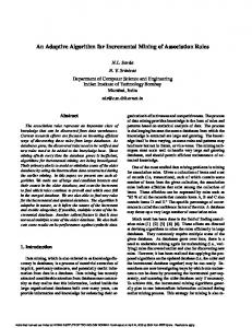
Fig. 1. NCBPP distribution as a function of TR distance.

Fig. 2. Allan deviation of NCBPP.

III. WIRELESS SENSOR CHANNEL ERROR CHARACTERISTICS

quires 2-byte correction code for 1-byte error. This static FEC algorithm, however, leads to 24-byte waste at TR distance less than 11 m where the maximum number of erroneous bytes is less than 6. Fig. 2 shows how fast the channel BER changes by plotting Allan deviation [9]. For Allan deviation, we divide a packet trace into time slots, compute NCBPP average of each time slot, and finally calculate Allan deviation, namely the variance of two neighbor time slots’ NCBPP. Allan deviation represents the smoothness of BER changes. Fig. 2 displays five Allan deviation graphs for five different TR distances as the time slot width for averaging NCBPP expands. In Fig. 2, the Allan deviation of 13 m trace is 4-byte at 1 s (second) time span while it rapidly decreases down to 1byte at 60 s interval. This Allan deviation plots again verify that NCBPP slowly changes at close TR distances while it abruptly varies at distant ones. This observation also illustrates the appropriate FEC code size difference between two adjacent FEC levels depends on the time scale to track down. When AFECCC aims at tracing 1 s BER variations, for example, its levels should be apart further than 4-byte at least. On the other hand, when it tries to follow long-term variations, the difference between two neighbor levels should be more than 4-byte. Figs. 3(a) and 3(b) show some visual evidence of AFECCC adaptability over sensor channels by depicting two average NCBPP variations of an 11 m trace when the average time span sets to 1 s and 10 s, respectively. These two figures perceptibly prove the existence of some low-frequency variations for AFECCC to faithfully trace down, especially like a wide deep valley between 700 s and 1200 s even though numerous spikes are dispersed over entire observation interval. Fig. 4 computes the ratio of theoretical waste time to the total observation interval when four static FEC algorithms are applied to the collected packet traces. Note that a static FEC algorithm wastes the bandwidth by transmission of its excessive FEC codes and packet losses due to its deficient FEC code strength. Four static FEC algorithms, FEC1, FEC2, FEC3, and FEC4 in Fig. 4 are assumed to add 6, 10, 20, and 40-byte RS code, respectively to recover 3, 5, 10, and 20 erroneous bytes. The code

This section examines the characteristics of bit errors in sensor networks to determine whether their BER varies smoothly enough to be traced down by an adaptive algorithm. When wireless channel is modeled as a state machine and a state is specified as BER, AFECCC adaptability is determined by the average duration of a state and the BER difference between two adjacent states. If BER varies more rapidly than the adaptation delay taken for detecting BER variation and calculating the suitable FEC level, it hardly accomplishes any improvement. If the channel BER is constant, furthermore, it may be useless. Fig. 1 shows the number of corrupted bytes per packet (NCBPP) standard deviation distribution of 10 traces at each TR distance (standing for the distance between the transmitter and receiver) by incrementing 1 m from 6 m to 13 m. Each trace represents 4-hour traffic from a sensor network where a Mica Mote sender continues to transmit 100-byte packets to its receiver at the maximum speed of 3.2 kbps by frequency shift keying (FSK) modulation with 915 MHz carrier signal and 90 mW transmission power. Fig. 1 indicates that the average NCBPP gradually increases from 2-byte within close distances less than 11 m to 11-byte as TR distance approaches 13 m, the threshold distance for distinguishing signal. The standard deviation range also widens from 2-byte up to 10-byte as TR distance gets larger. The growth of the average NCBPP as a function of TR distance is explained by large scale fading (LSF) effect that the signal power fades in proportion to TR distance. The expansion of the standard deviation span is due to that small scale fading (SSF) effect mainly caused by multi-path interferences gets stronger as the signal power becomes weaker. Based on Fig. 1, we can say that AFECCC is indispensable to accommodate the wide BER distribution when receivers move around or even when they are statically located apart further than 10 m from their sender. When a receiver roams around within 13 m radius from its sender, for instance, the sender needs to add 36-byte Reed-Solomon (RS) [8] code to correct the worst 18 damaged bytes at 13 m TR distance. Note that RS code re-

4

JOURNAL OF COMMUNICATIONS AND NETWORKS, VOL. 7, NO. 4, DECEMBER 2005

(a) Fig. 4. Bandwidth waste ratio of four static FEC algorithms.

(b) Fig. 3. NCBPP variation over two different time scales: (a) Average NCBPP per second variations, (b) average NCBPP per 10 second variations.

size of each FEC algorithm is decided based on the measured error distributions where damaged bytes of 90% corrupt packets range from 2 to 20-byte. In Fig. 4, at first IEEE 802.11 without any FEC algorithm spends more than 70% of transmission time due to heavy packet losses. FEC4 and FEC1 consume almost 37% and 4% of the total time for unnecessary extra FEC code transmission while wasting 0.2% and 8% for packet loss at 6 m TR distance. On the other hand, at 13 m these two algorithms spend 25% and 2% for FEC code overhead while 10% and 78% for packet drops. To minimize the bandwidth waste depicted in Fig. 4, wireless networks need to dynamically select FEC2 in [6 m, 10 m], FEC3 in [10 m, 12 m], and finally FEC4 around 13 m. IV. AFECCC ALGORITHM This section introduces AFECCC algorithm that gradually approximates a suitable FEC level among some available FEC levels matching to the underlying wireless channel BER only by the assistance of acknowledgment packet arrivals. It descends to the lower FEC level some time called drop timeout after consecutive acknowledgements successfully arrive while immediately ascending to the higher one at a packet loss. It continues

to adopt the previous starting FEC level until the drop timeout expires differently than the traditional hybrid Type-II dynamic algorithms [2], [4]. AFECCC incrementally infers the appropriate FEC level or the number of FEC code bytes for the next packet to use since receivers seldom estimate the exact number of corrupted bytes once the number of error bytes is beyond the correction capability of the attached FEC code. Senders also hardly deduce this number from SNR that are often measurable and fed back by their receivers. AFECCC joins at the higher FEC level at the detection of a packet loss. Since the overhead of transmitting additional extra FEC code is much smaller than that of an entire packet retransmission, adding more FEC codes is much better for improving the performance than taking a risk of dropping another packet. The accumulation of unnecessary FEC code transmissions during a long error-free period, however, unacceptably deteriorates the throughput. To determine the appropriate drop time to the lower level, AFECCC maintains a drop timer (DT ) for each level whose timeout is adjusted by a binary exponential back-off algorithm. Whenever it joins a new FEC level, it exponentially increases DT of this newly adopted level up to Tmax by multiplying with a multiplication factor α (> 1). The more frequently it visits a FEC level, the larger its drop timeout grows to be stable at this level. Notice that α and Tmax decide the polling frequency to check the channel status improvement, leading to the polling overhead of AFECCC. The smaller α, for example, the more frequently AFECCC evaluates the channel behavior by weakening the FEC code. AFECCC, furthermore, retains a global polling timer to decay DT s of the other levels except the currently adopted level. Whenever this global timer is expired every Tp , it shrinks the DT timeout value of the other levels up to Tmin by multiplying with a decay factor, β (< 1). This decay operation has an effect of incrementally forgetting the old channel status as time goes by. In summary, Fig. 5 illustrates these transitions among some predetermined levels of AFECCC. The AFECCC four tunable variables, α, Tmax , Tmin , and β

AHN et al.: AN ADAPTIVE FEC CODE CONTROL ALGORITHM FOR MOBILE...

DT1 DTk DTk

1

DTk

1

,

DT1 1

DTk

1

, DTk -1 ,

, DTn

DTk -1

FEC level

,

DTn DTk

TP timeout

DTk timeout

(K-1)-th level

DTk

DTk+1 timeout

K-th level

(K+1)-th level

Packet drop DTk

5

Packet drop

DTk

DTk

1

DTk

1

Fig. 5. State transition diagram of AFECCC.

RTT+backoff

n

RTT+backoff

determine the frequency of channel examinations. The smaller these four variables, the more aggressively AFECCC reduces the FEC code size at the expense of retransmission. Heuristically, we approximately set Tp , Tmin , Tmax to round trip time (RT T ), hRT T , hTmin , respectively when the code size gap between two neighbor levels is 1/h of the packet size. Precisely, AFECCC adjusts DT of other levels except the current on whenever one RT T for successfully sending a packet elapses. It also sets the earliest drop timeout Tmin , to h × RT T taken for h packets to be sent. Note that h×RT T is the duration for the total accumulated overhead of extra FEC code transmissions 1/h(h × RT T ) to be equal to the waste time due to a packet loss. With this value, AFECCC can test the channel before the FEC overhead becomes greater than the retransmission overhead.

RTT+backoff Time RT T (a)

FEC level

2log 2 n DT

c c .. c

22

n 1

2

RTT+backoff

V. AFECCC ALGORITHM ANALYSIS

Time

This section tries to determine an appropriate transition combination by theoretically analyzing the performance of four possible level change schemes, additively increase (AI), multiplicatively increase (MI), additively decrease (AD), and multiplicatively decrease (MD) ways. A. Two Upward Transition Method Fig. 6 pictorially depicts the behavior of two upward transition techniques when the channel BER jumps up to what n-th FEC level deals with as the dotted line depicts in Fig. 6. Equation (1) shows the AI upward overhead, namely the time taken to ascend to n-th FEC level by repeating n-time retransmissions. Note that the worst k-th average retransmission time is the sum of backoff delay 2k−1 Ts and RT T where Ts is the minimum delay for avoiding collision and Ts is set to 50 ms in our sensor network. RT T is the time to finish transmissions of RTS, CTS, DATA, and ACK packets when IEEE 802.11 networks employ the virtual channel sensing. Otherwise, RT T is the time to finish transmissions of DATA and ACK packets. Uoverhead = RT T × n +

n X

RT T (b) Fig. 6. Two upward transition schemes: (a) Additive-increase, (b) multiplicative-increase.

denotes the wasted time for sending extra FEC codes before descending to n-th level in AD way. Note that the k-th (> n) level attaches C(k − n) excessive bytes at each packet during DT duration under the assumption that each FEC level is evenly spaced by C-byte FEC code and the underlying wireless channel’s bandwidth is BW . The total overhead of extra FEC code is the multiplication of C(k − n)/BW , the transmission time of a packet’s extra code at the k-th level and DT /RT T , the number of packets sent before DT expires. log2 n

Uoverhead = RT T log2 n +

X

k=1 n X

(C(k − n)/BW )

k=2log2 n

2k−1 Ts .

2k−1 Ts + DT . RT T

(2)

(1)

k=1

B. Two Downward Transition Method log2 n

retransmissions In contrast to AI technique, MI needs 2 to reach above n-th level shown in Fig. 6 (b). The first and second terms in (2) represent the overhead of these retransmissions. Note that the ceiling-bar of log2 n is an operator rounding up a float number. When n is not the exponent of 2, the third term

Fig. 7 graphically depicts the behavior of two downward transition techniques when the current BER jumps down from (m + n)-th level to m-th one where m is an arbitrary number. Equation (3) computes the AD overhead, in which the first term indicates the transmission time for additional FEC codes

6

JOURNAL OF COMMUNICATIONS AND NETWORKS, VOL. 7, NO. 4, DECEMBER 2005

FEC level

MD is more dominant than in MI and AD, respectively. So like in 802.11 networks where a packet retransmission takes more time than the transmission of FEC code, generally AFECCC is safe to employ a pair of AI and MD to dynamically adjust the amount of FEC code.

DT

c c .

DT

n c c …...

c VI. THEORETICAL MODELS FOR WIRELESS CHANNEL RT T Time

(a)

FEC level DT

c … c

21

DT

n c

c

…

2log 2 n RTT+backoff RT T Time (b) Fig. 7. Two downward transition schemes: (a) Additive-decrease, (b) multiplicative-decrease.

before going down to (m − 1)-th level and the second term amounts to a packet retransmission time caused for going up from (m − 1)-th level to m-th one under the assumption that AFECCC transits in AI way. Doverhead =

n X

(C(n − k)/BW )

k=0

DT + RT T. RT T

(3)

Equation (4) calculates the MD overhead, in which the first term explains the overhead of additive FEC codes before exponentially descending to (m + (n − 2log2 n ))-th level when n is not the exponent of 2. The second and third terms indicates the upward overhead of AI going up from (m + (n − 2log2 n ))-th to m-th under the assumption that AFECCC goes up in AI way. log2 n−1

Doverhead =

X

(C × (n − 2k )/BW ) ×

k=0

(2

log2 n

− n)RT T +

DT + RT T

2 n −n 2logX

This section introduces two approaches to model bit-level propagation errors in packet-level network simulators [10], [11]. First, analytical channel models specify physical wireless signal propagation phenomena known as large-scale fading (LSF) and small-scale fading (SSF) effects. ns-2 [11], for example, includes three LSF models (free space model, two-ray ground reflection model, and shadowing model) and one SSF model (Ricean distribution) [12]. These physical models allow ns-2 to compute the average signal power of every packet arrived at a receiver and based on the comparison of the perceived signal power to the receiving threshold, determine packet drops. Since this approach assumes the same signal power sustained all the way during a packet’s transmission duration, however, it can’t accurately predict that the error probability grows in proportion to the packet size. To overcome this problem, Holland [7] calculates a packet’s signal power several times whenever the theoretical SSF duration expires if the packet transmission lasts longer than the SSF interval. Still this approach can’t provide fine granularity for the number of corrupt bits and their locations needed for evaluating FEC algorithms. Differently from imitating physical phenomena, the second one statistically defines observed wireless behaviors with some mathematical equations. This category, for example, contains Gilbert Elliot (GE) [13] model also known as two-state Markov chain and chaotic map (CM) [14] which many researchers [5], [15] have adopted in studying link-level ARQ and FEC performance. They are popularly employed in packet simulators since they faithfully represent the typical wireless biterror burstiness by assuming two states each of which represents short-term heavy BER and long-term light BER, respectively. Especially, CM model strictly expresses burstier error characteristics of 802.11 LAN than what GE model represents. It transits between the good state with no error and the bad state with error by (5) which computes Xt+1 at each bit transmission. When the Xt+1 is greater than 1, it assumes no error. Otherwise it generates one error bit. Three variables z, u, and e in (5) determine transition frequency between two states, the probability of staying in the current status, and the maximum number of bit strings in a given state, respectively. Xt+1 = Xt + µXtz + ², t ∈ N.

k

2 Ts .

(4)

k=0

As calculated in the above four equations, the performance of these four transition techniques depends on several parameters such as channel propagation error characteristics, FEC code size, RT T , DT timeout, etc. Even though we hardly quantitatively compare the four equations due to various parameters, we can roughly say that the packet loss overhead term in AI and

(5)

When error bit distributions can’t be accurately summarized as some mathematical equations, the second approach uses table-driven or trace-driven methods [16] storing every details of real traffic. The table-driven one builds a histogram which records the probability values for each error bit strings from collected traces. The trace-driven way exactly replays error byte counts collected from real traces or channel simulators [17], [18]. Even though the last one limits the number of packets

AHN et al.: AN ADAPTIVE FEC CODE CONTROL ALGORITHM FOR MOBILE...

7

IEEE 802.11 MAC RS(106,100) RS(112,100) RS(118,100) RS(126,100) LA/IR Type2 Recursive LA/IR AFECCC

Fig. 8. Performance of four transition algorithms. Fig. 9. AFECCC performance in Markov chain.

to simulate by trace size, it has an advantage to precisely model a specific channel. This paper adopts three channel models, GE, CM, and real sensor traces for evaluating AFECCC performance. VII. EVALUATION This section evaluates the performance of four adaptation methods (AIAD, AIMD, MIAD, MIMD), compares AFECCC throughput with that of static and conventional dynamic FEC algorithms, and finally measures AFECCC performance over real sensor networks. Note that the performance only counts the number of packets that are received successfully or recovered with their FEC code. The successful recovery is determined by the attached error detection code such as cyclic redundancy code (CRC). A. The Performance Analysis of Four Transition Schemes Fig. 8 shows the ratio of four transition methods’ performance measured over noisy channels to the best performance over an error-free channel when a sender constantly transmit 100-byte packets over 512 kbps channel of an IEEE 802.11 network. Its three axes z, y, x represent the performance ratio, the duration of a given BER state as an unit of second, and BER when the noisy channel is modeled by two-state Markov chains. Namely the good state and bad state are defined as (x, y) and (0, y). Five parameters of AFECCC, α, β, Tmax , Tmin , Tp are set to 2, 0.8, 1000 ms, 60 ms, 6 ms where 6 ms is one RTT of this 802.11b network. Finally, we assume that AFECCC maintains 11 FEC levels each of which corrects 2, 5, 8, 12, 16, 21, 26, 33, 40, and 45 contaminated bytes. Fig. 8 indicates that the performance of the four algorithms is strongly affected with the channel BER duration as BER increases. In detail, they achieve almost the same throughput with low BER from 0 up to 0.02 regardless of BER duration while as BER becomes larger and the channel state changes rapidly, MIAD performs better nearly by 50% than the other three schemes. It is due to that it minimizes the packet loss by adapting quickly to the bad state but slowly to the good state.

B. The Performance Comparison of AFECCC to Static and Two Previous Dynamic FEC Algorithms Fig. 9 compares the performance of AFECCC to that of four FEC algorithms, RS(106, 100), RS(112, 100), RS(118, 100), RS(126, 100) [8] and two dynamic ones named LA-IR II and retrace recursive LA-IR [2] when two states of Markov chain are set to (0, 20 ms) and (x, 20 ms) in the same network as the one for Fig. 8. Note that RS(u, w) means w data symbols and (u − w) correction RS symbols where (u − w) correction symbols restore (u − w)/2 corrupt symbols. For Fig. 9, we set a symbol to one byte and configure AFECCC to dynamically choose one among these four static codes RS(106, 100), RS(112, 100), RS(118, 100), and RS(126, 100). For computing the starting level in retrace recursive LA-IR, we pick the most successful level among ten previous successful levels. Each graph of Fig. 9 plots the ratio of one algorithm’s performance to the maximum achievable throughput over the error-free channel and each dot on a graph averages five simulation results. Fig. 9 shows that ARQ performance quickly falls off to zero as the bad state’s BER approximates to 10−3 , where every 100byte packet is likely to be inflicted with one-bit error. The four static FEC codes maintain constant throughput with 20% maximum difference among them before x becomes 10−2 where each performance sharply drops. Especially the performance of RS(126, 100) is less by 20% than any static codes but runs constant all the way before 10−1 where the others’ performance reaches almost zero. Fig. 9 illustrates that AFECCC orderly traces the behavior of 802.11, RS(106, 100), RS(112, 100), RS(118, 100), and RS(126, 100) during [0, 0.03], [0.03, 0.06], [0.06, 0.09], [0.09, 0.13], and [0.13, 0.15] interval of x-axis. AFECCC, however, performs less by 5% than the best static algorithm in each interval due to its adaptation overhead. It adapts to the BER changes similarly as the two dynamic LA-IR algorithms even though it performs 10% better after BER grows greater than 10−4 . Note that the two performance graphs of two LA-IR schemes are almost indistinctly overlapped. Furthermore, the two algorithms’ performance rapidly drops to almost 10% while

8

JOURNAL OF COMMUNICATIONS AND NETWORKS, VOL. 7, NO. 4, DECEMBER 2005

IEEE 802.11 MAC

RS(106,100) RS(112,100) RS(118,100) RS(126,100) LA/IR Type2 Recursive LA/IR AFECCC

Fig. 10. AFECCC performance in chaotic map.

AFECCC maintains 50% performance ratio as BER approaches 10−1 . The reason of AFECCC’s superiority in this heavy BER range is mainly due to the multiplicative increase rate which can rapidly adapt to wide BER fluctuations. Fig. 10 also evidences the performance of the eight algorithms under the same environment as Fig. 9 except that CM model is adopted for wireless channels. As like Figs. 9 and 10 predicts that each static code maintains constant throughput before its threshold BER at which almost every packet is damaged too heavily to be corrected. In contrast to Fig. 9, however, their performance smoothly degrades at its BER threshold since CM model is burstier than two-state Markov chain. Namely under the same average BER, CM model produces the same amount of error bits for the shorter duration than two-state Markov chain. Due to the high degree of burstiness, they successfully transport more packets under the same BER than in Fig. 9. AFECCC achieves better in CM model by 3% than in twostate Markov chain and even accomplishes better by 5% than any other static algorithms at around 2 × 10−2 BER. It is due to that in CM model the good state sustains longer so that AFECCC suffers less packet loss than in two-state Markov chain whenever it switches to the lower FEC level. It also achieves better performance than two LA-IR algorithms as BER becomes greater than around 2 × 10−3 due to the reason explained in Fig. 9. Fig. 11 evaluates the performance of eight FEC algorithms over real traces collected from a real sensor network where a sender transmits 100-byte packets to its receiver while increasing TR distance from 1 m to 13 m. For emulating the receiver’s movement, we appropriately mix 10-minute packet traffic from different traces measured at different locations for a given average BER depicted at x-axis. In contrast to Fig. 10, Fig. 11 indicates that the performance of the eight algorithms falls earlier before their predicted threshold since propagation errors in these artificially interleaved traces are more randomly and uniformly distributed. Fig. 11 also shows that the performance of AFECCC is located in the middle of RS(118, 100) and RS(126, 100) in [10−3 , 1.3 × 10−2 ] BER

IEEE 802.11 MAC

RS(104,100) RS(108,100) RS(120,100) RS(140,100) LA/IR Type2 Recursive LA/IR AFECCC

Fig. 11. AFECCC performance in real trace. Table 1. The number of retransmitted bytes and FEC bytes per packet at each BER.

802.11 MAC RS(104,100) RS(108,100) RS(120,100) RS(140,100) LA-IR Type II Retrace recursive LA-IR AFECCC

0.001 0.012 0.052 0.079 0.097 21.5 290.8 526.6 980.2 4852.8 7.1 81.1 228.7 478.7 1255.0 11.2 15.5 77.9 192.0 339.4 25.2 25.2 60.8 101.5 134.7 52.2 52.2 70.0 86.0 96.3 19.7 104.9 152.3 187.7 218.9 19.8

126.1 225.0 294.0

340.2

16.9

29.2

102.6

62.7

87.6

range and follows that of RS(126, 100) as x approaches 10−1 . At 4.6×10−2 BER, AFECCC’s performance drops sharply even though it is still better than RS(118, 100) by 5%. The reason of AFECCC’s deep fall at this BER comparing to the next 5.2 × 10−2 BER would be that more packets in this trace file are tainted than in 5.2 × 10−2 trace by 8% even though 5.2 × 10−2 trace file’s BER is higher than 4.6 × 10−2 BER. The packet BER of 4.6 × 10−2 trace file is also somewhat randomly fluctuated between what RS(118, 100) and RS(126, 100) can recover so that AFECCC is hard to be stable at RS(126, 100). Finally, AFECCC performs better than the two LA-IR algorithms over the entire BER interval. It is also due to that the LA-IRs fail to predict the right starting FEC level and swiftly adapt to the wide BER change by additively increasing the FEC level rather than multiplicatively. C. AFECCC Implementation and Performance Analysis Table 1 shows the average number of retransmitted bytes plus FEC bytes sent by the eight algorithms to successfully forward a packet at five BERs used in the experiment for Fig. 11. The top row and the leftmost column of Table 1 list five BERs at which each algorithm’s overhead is evaluated and the type of FEC algorithms, respectively. Table 1 indicates that the overhead of AFECCC approximates to the second least among those

AHN et al.: AN ADAPTIVE FEC CODE CONTROL ALGORITHM FOR MOBILE...

Octets:

2

Frame Control

2

6

6

Duration

Dest addr

Src addr

9

6

2

1

variable

BSSID

Sequence control

FEC strength

variable

Data

FEC

Data packet frame Octets:

2

Frame control

2

6

6

4

Duration

Dest addr

Src addr

FEC

2

2

6

4

Duration

Dest addr

FEC

RTS frame Octets: 2 Frame control

2

6

Duration

Dest addr

4 FEC

CTS frame

Octets:

Frame control

ACK frame

Fig. 13. Four extended packet formats for AFECCC.

SMAC.C Polling timer

Carrier sense control back-off and retry

MAC layer

Drop timer

RTS/CTS/ACK Packet drop timer

Phy_FEC_timer_fire

Reset timer

Phy_Tx_fail

Tx_pkt

Successful ACK arrival

Rx_pkt Tx_pkt_done

Phy_drop_timer_fire

Free_processing_buffer

PHY_RADIO.C CRC check Physical layer

Decrease drop timer

Decrease FEC

Increase FEC

MIAD FEC control

RADIO_CONTROL.C

FEC encoding/decoding Byte spooling/buffering

CODEC_MANCHESTER.C

Radio control carrier sense

Encoding/decoding

Fig. 12. AFECCC implementation at SMAC.

Fig. 14. Performance ratio of four static FEC codes to AFECCC.

of the static FEC algorithms in each low BER column and at least takes a few tens of bytes fewer than the other static and the two dynamic LA-IR algorithms. Based on the total transmission overhead over the entire BER range, we believe that AFECCC is energy-efficient more than the static FEC and LA-IR algorithms even though it executes around some tens of instructions per packet. Note that the transmission of one byte tends to consume more energy than the execution of a few instructions as T-R distance gets larger. Fig. 12 illustrates AFECCC implementation [19] in sensorMAC (SMAC) [20] that is quite similar to 802.11 except that for power saving receivers sleep whenever they have no data to receive. As shown in Fig. 12, AFECCC integrates four event handlers for processing DT timeout, P T timeout, packet drop detection timeout, and successful acknowledgement arrival at SMAC layer while it puts RS FEC encode and decode functions at its physical layer. Fig. 13 also lists four extended headers of RTS, CTS, ACK, and Data frames to carry FEC code for AFECCC. Since the three control packets RTS, CTS, and ACK are relatively short, we assume that their FEC code is of fixed size while data frames

reserve two fields to store FEC code size in their header and the corresponding FEC code at their trail. Fig. 14 draws the ratio of four static FEC codes performance to that of AFECCC when a Mica Mote transmits 80-byte packets for 2-hour by varying TR distance from 1 m to 11 m. For the fair comparison of the five algorithms, we compute each static FEC performance when the four static FEC algorithms are assumed to work over the same packet traffic experienced by AFECCC. Namely, we calculate the waste time of packet losses and extra code transmission when the same degree of corruption occurs to the four static algorithms. It is due to that since the sensor channel widely varies, we hardly produce the same live networks for fair comparison. Each point of four graphs in Fig. 14 represents the average over three AFECCC traces. Fig. 14 shows that the performance graph of weak RS(84, 80) crosses those of three strong codes, RS(88, 80), RS(92, 80), and RS(100, 80) as TR distance increases as predicted in the above simulation experiments. It also proves that AFECCC performs better in all TR distances even though RS(88, 80) and RS(92, 80) achieve almost the same performance as AFECCC as TR distance approaches 11 m.

10

JOURNAL OF COMMUNICATIONS AND NETWORKS, VOL. 7, NO. 4, DECEMBER 2005

VIII. CONCLUSION This paper provides some evidences that low-power sensor channels’ BER tends to smoothly vary to dynamically adjust the FEC code size for improving the sensor network performance. It also proposes an adaptive FEC code control algorithm called AFECCC and evaluates its performance under various channel models and over real sensor networks. AFECCC dynamically matches the FEC code size to the low-frequency wireless channel BER, which is evaluated by acknowledgement packet arrivals. According to the simulations with various theoretical channel models and live experiments over sensor networks, AFECCC performs better than any static FEC algorithms and some conventional dynamic FEC algorithms. We will try to devise a technique to automatically determine the tunable variables of AFECCC based on its applied network environments. Finally, we also plan to accurately quantify the energy saved by AFECCC under simulations and real mobile sensor networks. REFERENCES [1] [2]

[3] [4] [5] [6] [7] [8] [9] [10] [11] [12] [13] [14] [15] [16] [17] [18]

[19]

J. Heidemann, F. Silva, C. Intanagonwiwat, R. Govindan, D. Estrin, and D. Ganesan, “Building efficient wireless sensor networks with low-level naming,” in Proc. SOSP 2001, vol. 35, no 5, Oct. 2001, pp 146–159. A. Levisianou, C. Assimakopoulos, F.-N. Pavlidou, and A. Polydoros, “A recursive IR protocol for multicarrier communications,” in Proc. 6-th International OFDM-Workshop, Hamburg, Czech Republic, Sept. 2001, pp. 22-1–22-4. J. Hagenauer, “Rate compatible punctured convolutional codes (RCPC codes) and their applications,” IEEE Trans. Commun., vol. 36, no 4, pp. 389–400, Apr. 1988. L. Zhao, J. W. Mark, and Y. C. Yoon, “A combined link adaptation and incremental redundancy protocol for enhanced data transmission,” in Proc. GLOBECOM 2001, San Antonio, Texas, Nov. 2001, pp. 25–29. P. Lettieri and M. B. Srivastava, “Adaptive frame length control for improving wireless link throughput, range, and energy efficiency,” in Proc. INFOCOM’98, Apr. 1998, pp. 564–571. G. Wu, C.-W. Chu, K. Wine, J. Evans, and R. Frenkiel, “WINMAC: A novel transmission protocol for infostations,” in Proc. VTC’99, May 1999, pp.1340–1344. G. Holland, N. Vaidya, and P. Bahl, “A rate-adaptive MAC protocol for multi-hop wireless networks,” in Proc. ACM SigMobile, July 2001, pp. 236–250. W. Peterson and E. Weldon Jr., Error-Correcting Codes, 2nd ed., The Massachusetts Institute of Technology. D. W. Allan, “Time and frequency (time domain) characterization, estimation, and prediction of precision clocks and oscillators,” IEEE Trans. Ultrason., Ferroelect., Freq. Contr., vol. 34, no. 6, Nov. 1987. M. Takai, R. Bagrodia, A. Lee, and M. Gerla, “Impact of channel models on simulation of large scale wireless networks,” in Proc. MSWiM’99, Aug. 1999, pp. 7–14. Network Simulator NS-2, available at http://www.isi.edu/nsnam/ns. R. J. Punnoose, P. V. Nikitin, and D. D. Stancil, “Efficient simulation of Ricean fading,” in Proc. VTC 2000, Sept. 2000, pp.764–767. E. N. Gilbert, “Capacity of a burst-noise channel,” Bell Syst. Tech. J., vol. 39, pp 1253–1266, Sept. 1960. A. Kpke, A. Willig, and H. Karl, “Chaotic maps as parsimonious bit error models of wireless channels,” in Proc. INFOCOM 2003, vol. 22, no. 1, Mar. 2003, pp. 513–523. M. Zorzi, “Performance of FEC and ARQ error control in bursty channels under delay constraints,” in Proc. VTC’98, May 1998, pp. 1390–1394. A. Kumar and R. Gupta, “Capacity evaluation of frequency hopping based ad-hoc systems,” in Proc. SigMetrics 2001, June 2001, pp. 133–142. C. M. Keller, Generic Channel Simulator, MIT Lincoln Laboratory Project Report AST-46, Aug. 1997. T. S. Rappaport, S. Y. Seidel, and K. Takamizawa, “Statistical channel impulse response models for factory and open plan building radio communication system design,” IEEE Trans. Commun., vol. COM-39 no. 5, pp. 794–806, May 1991. Available at http://network.dongguk.ac.kr/publication/AFECCC/AFECCC .html.

[20] W. Ye, J. Heidemann, and D. Estrin, “An energy-efficient MAC protocol for wireless sensor networks,” in Proc. IEEE INFOCOM 2002. June, 2002, pp. 1567–1576.

Jong-Suk Ahn received the Ph.D. degree and the M.S. degree in electrical engineering from the University of Southern California in 1995 and from the Korean Advanced Institute of Science and Technology in 1985, respectively and the B.S. degree from Seoul National Univerisity in 1983. He was a visiting researcher in ISI/USC for one year from 2000. He was awarded Gaheon Prize for the best paper in 2003 from the Korean Information Science Society. He is currently an associate professor at the Dongguk University in Korea. His major interests are in sensor networks, dynamic error control and flow control algorithms over wireless Internet, fast IP routing techniques, and network simulation techniques.

Seung-Wook Hong was born in Hwaseong, Korea, on April 23, 1977. He received the B.S. degree in Information and Communication Engineering and the M.S. degree in Computer Engineering from the Dongguk University of Seoul, Korea, in 2003 and 2005, respectively. He is currently a computer engineer at the SAMSUNG Electronics Corp. in Korea. His major interests are in embedded systems, sensor networks, 802.11 MAC protocol, and device driver programming.

John Heidemann is a senior project leader at USC/ISI and a research associate professor at USC in the CS Department. At ISI he leads I-LENSE, the ISI Laboratory for Embedded Networked Sensor Experimentation, and investigates networking protocols and traffic analysis as part of the ANT (Analysis of Network Traffic) group. He received his B.S. from University of Nebraska-Lincoln and his M.S. and Ph.D. from UCLA, and is a member of ACM and Usenix, and a senior member of IEEE.