1294
JOURNAL OF ATMOSPHERIC AND OCEANIC TECHNOLOGY
VOLUME 22
An Advanced Method to Estimate Deep Currents from Profiling Floats JONG JIN PARK
AND
KUH KIM
School of Earth and Environmental Sciences, Seoul National University, Seoul, Korea
BRIAN A. KING Southampton Oceanography Centre, Southampton, United Kingdom
STEPHEN C. RISER School of Oceanography, University of Washington, Seattle, Washington (Manuscript received 10 October 2003, in final form 19 November 2004) ABSTRACT Subsurface ocean currents can be estimated from the positions of drifting profiling floats that are being widely deployed for the international Argo program. The calculation of subsurface velocity depends on how the trajectory of the float while on the surface is treated. The following three aspects of the calculation of drift velocities are addressed: the accurate determination of surfacing and dive times, a new method for extrapolating surface and dive positions from the set of discrete Argos position fixes, and a discussion of the errors in the method. In the new method described herein, the mean drift velocity and the phase and amplitude of inertial motions are derived explicitly from a least squares fit to the set of Argos position fixes for each surface cycle separately. The new method differs from previous methods that include prior assumptions about the statistics of inertial motions. It is concluded that the endpoints of the subsurface trajectory can be estimated with accuracy better than 1.7 km (East Sea/Sea of Japan) and 0.8 km (Indian Ocean). All errors, combined with the error that results from geostrophic shear and extrapolation, should result in individual subsurface velocity estimates with uncertainty of the order of 0.2 cm s⫺1.
1. Introduction The rapidly developing array of floats in the Argo program is now providing over 3000 ocean profiles per month, and is planned to increase to a global distribution of over 100 000 profiles per year. While the use of Argo ocean profiles is widely discussed, much less attention has been given to the subsurface drift velocity associated with each profile. The Autonomous Lagrangian Circulation Explorer (ALACE), the predecessor of the present generation of profiling floats, was originally developed to measure deep currents in a Lagrangian way (Davis and Zenk 2001; Davis et al. 1992). However, there are still rather few examples of using ALACE and subsequent models
Corresponding author address: Jong Jin Park, Ocean Circulation Research Laboratory, School of Earth and Environmental Sciences, Seoul National University, San 56-1, Sillim-dong, Kwanak-gu, Seoul 151-742, Korea. E-mail:
[email protected]
© 2005 American Meteorological Society
JTECH1748
of floats to estimate deep currents. This is partly a result of uncertainty in converting float position fixes to subsurface currents. After a float rises from its parking depth and reaches the sea surface, it drifts an unknown distance at the surface before its position is determined by an Argos satellite. Similarly, floats drift away after their last contact with a satellite before they start to dive. In principle, deep currents are estimated by dividing the distance that the floats move at parking depths by the duration of drift, which requires knowledge of the time and positions of the diving and surfacing. This critical information is not directly measured for most floats. Because currents are much stronger at and near the surface than at parking depths, the unknown drift before the first fix and after the last fix, while floats are at the surface, provide a significant source of error in estimating the deep currents. In this paper, we present a new method for extrapolating sets of Argos float position fixes to the surfacing and diving locations, demonstrating explicitly the importance of a good representation of inertial motions in
AUGUST 2005
1295
PARK ET AL.
the extrapolation procedure. An important aspect of determining the surface and dive positions is fixing the time of these events as accurately as possible. We describe how this can be done. While the procedure is not difficult, it does not seem to be well documented or widely circulated. Finally, we present an analysis of the uncertainty in position fixing using the proposed method. The data used in this paper are from 36 floats deployed in the East Sea/Sea of Japan (hereafter EJS) for the Korea–U.S. Circulation Research on the East Asian Marginal Seas (CREAMS) program and set to drift at 800 m. The period covered is from July/August 1999 to March 2002. We also use data from 24 floats deployed near 32°S in the Indian Ocean (hereafter IO) by the United Kingdom for the international Argo program, and set to drift at 2000 m; the majority of these floats were deployed in March/April of 2002. All of the floats considered are autonomous profiling explorer (APEX) floats built by Webb Research Corporation, reporting positions via Argos.
2. Estimation of subsurface velocity a. Reference time A float starts its first cycle as it dives at time T 1desc_start in Fig. 1, which is called the reference time TR in this paper for a reason that will become clear. Upon reaching its parking depth at T 1desc_end, the float moves with deep currents until it starts ascending at T 1asc_start, which is determined by the preset time interval ⌬Tdown after T 1desc_start. This time interval is referred to as the “DOWN time” in an APEX float, and was 168 h (7 days) for the profiling floats deployed in the EJS, and 228 h for the United Kingdom IO floats. The float arrives at the sea surface at T 1asc_end and drifts with the surface current while its positions are fixed by satellite several times at T 11, T 12, . . . , T 1n. To allow for the transmission of data via Argos satellites, the float stays at the surface for several hours. The float begins its next cycle at T 2desc_start as it starts diving again. The second diving time, T 2desc_start is also preprogrammed and occurs ⌬Tup after the start of ascent at T 1asc_start. The interval ⌬Tup is the APEX float “UP time,” and was 18 h for the floats in the EJS and 12 h in the IO. So, the float repeats its cycle with a period of ⌬Tcyc ⫽ ⌬Tdown ⫹ ⌬Tup. Other more complicated APEX missions are possible, and involve parking at a depth that is different from the maximum, or profiling to different depths on different cycles. The current at the parking depth for the first cycle can be estimated by dividing the distance the float moved between T 1desc_end and T 1asc_start by (T 1asc_start ⫺
T 1desc_end). However, these times and corresponding positions are not directly reported. The closest approximation for this estimate is to calculate the velocity vector between the two times T 1desc_start and T 1asc_end. Unfortunately, both T 1desc_start and T 1asc_end are sometimes not logged, and the positions corresponding to these times are not available either. While it is reasonable to expect that T 1desc_start should be available from good record keeping for floats deployed by a research vessel (though maybe not for floats deployed by ships of opportunity), and while it should be possible to infer this time from data reported in the APEX test message before the first dive, we note that the first dive time is quite often absent in files held by the Argo Global Data Assembly Centers. The surfacing time, or time of first transmission (which is earlier than the time when the first data are received via Argos, unless an Argos satellite happens to be passing over as the float arrives at the surface), is also sometimes missing. In this paper we report a way to determine the reference time TR, which is the first diving time T 1desc_start. Knowing this reference time, it is possible to determine the subsequent diving and surfacing times. Because a float repeats its cycle, we can take advantage of its exact period of operation ⌬Tcyc. If m is the cycle number, we consider the set of the last transmission time (T m last) for each cycle (Fig. 1c, red symbols), mapped back through m complete cycles, to a time just m before TR: T m RL ⫽ T last ⫺ ⌬Tcyc m, for each cycle. The upper envelope of this set is a lower bound on the reference time TR (Fig. 1b). Suppose we know the time that is taken for ascent from the parking depth to the surface ⌬Tasc. As discussed below, ⌬Tasc can be estimated from the manufacturer’s data, or calculated from the APEX data messages. We now consider the set containing the first fix for each cycle (Fig. 1c, blue symbols; T m first). These times are mapped back through (m ⫺ 1) complete cycles, with a further subtraction of the time corresponding to the final submerged period m (descent, drift, ascent). The set becomes T m RU ⫽ T first ⫺ m ⌬Tcyc (m ⫺ 1) ⫺ (⌬Tdown ⫹ ⌬Tup) where T RU is the upper limit of the reference time. The lower envelope of this set is an upper bound on the reference time TR. m Then T m RL ⬍ TR ⬍ T RU, as shown in Fig. 1b, and the range of TR becomes smaller as the number of cycles increases. Generally about 30 cycles are necessary to reduce the range of TR to within tens of minutes. After a sufficient number of cycles, TR can be determined as the midpoint between TRU and TRL.
1) CLOCK
JUMPS
We noted above that, in principle, and with careful record keeping, the details of the reference time TR,
1296
JOURNAL OF ATMOSPHERIC AND OCEANIC TECHNOLOGY
VOLUME 22
FIG. 1. (a) Schematic diagram of depth vs time for a float cycle. (c) The time of the first and last fix for each cycle, mapped back to the first cycle by subtracting the float cycle period. (b) The times from (c) have been mapped around the initial dive, so that the reference time can be calculated. The units are Julian day (starting on 1 Jan 1999).
dive times, and surface arrival times can all be calculated from the Argos messages, by assuming a uniform cycle period ⌬Tcyc. However, we have found that some monitoring of the transmission times following the procedure described above is advisable. Figure 2 shows the
Fig 1 live 4/C
equivalent plot to Fig. 1b for APEX float number 259. For cycles 26–59, there were neither position fixes nor a data broadcast. When the float returned to broadcasting at cycle 60, a jump in the reference time was evident and a new reference time is required for subsequent
AUGUST 2005
1297
PARK ET AL.
in incorrect estimates of the dive time and, therefore, incorrect estimates of the dive position.
2) DETERMINATION
FIG. 2. An example of the reference time estimation. In this case, the float stopped broadcasting after cycle 25. When it started broadcasting again at cycle 60, the reference time had changed by 2.8 h. The unit is Julian day (starting on 1 Jan 1999).
cycles. The offset of the reference time was 2.8 h. The new reference time can only be calculated from the times of the ARGOS messages. Failure to detect the jump and determine the new reference time will result
OF
⌬TASC
The time taken for a float to ascend from its parking depth to the surface ⌬Tasc can be estimated from the maximum depth and a constant ascending velocity that is specified by the manufacturer. For floats in the EJS, ⌬Tasc is close to 2.8 h. However, the surface arrival time, or at least the time of start of Argos transmissions, can be determined from data in the Argos messages. The message number 1 of an APEX transmission contains a counter of the number of times that message has been transmitted. Because the time of receipt of the Argos messages is known, if the ARGOS repetition rate is R seconds, if the APEX profile consists of M messages, and if the Nth copy of message 1 is received at time T, then the first ARGOS message was broadcast at a time T ⫺ (RM )(N ⫺ 1). Once the reference time TR has been determined, then the dive time for cycle number m is TR ⫹ (m ⫺ 1)⌬Tcyc. Therefore, we know or can calculate both the surface arrival time and the surface departure time. Because the total time for ascent plus surface drift ⌬Tup is known, we can calculate the duration of ascent ⌬Tasc. We have compared the actual ascent duration with that predicted from drift depth and assumed a uniform ascent rate. For the EJS floats we find a significant seasonal variation. Figure 3 shows the variation of the actual surface arrival time compared with the predicted arrival time. The variation is up to 2000 s, with later
FIG. 3. Difference between actual surface arrival time (time of first broadcast, calculated from engineering data) and predicted time, based on uniform ascent rate. Four different floats in the EJS show the same seasonal variation, and the same slow trend equivalent to about 1 s day⫺1.
Fig 2 3 live 4/C
1298
JOURNAL OF ATMOSPHERIC AND OCEANIC TECHNOLOGY
arrivals in summer a result of the more buoyant surface layer. The seasonal variation at 32°S in the IO was less significant. The trend in Fig. 3 suggests a systematic clock drift of about 370 s yr⫺1. Two years after deployment, floats are arriving at the surface 700 s earlier than programmed arrival time. Thus, the reference time should be recalculated every 40 to ⬃50 cycles to reduce the surfacing and diving time error by clock drifts.
3) SURFACING
AND DIVING TIME
In general, the dive time can be estimated from the first dive time (as power-on time plus delay of first dive time) and cycle period, and the surface arrival time can be determined from the metadata in the Argos messages, as mentioned above, if there is no clock drift or jumps, and if the first dive time and metadata are available. Otherwise, the reference time must be calculated, instead of using the first dive time. For instance, because the metadata of the floats in the EJS are available, the surface arrival time is calculated from the Argos messages. However, because of clock drifts, clock jumps, and no first dive time, the reference time that is newly obtained every 50 cycles provides more precise estimates of dive times.
b. Surfacing and diving positions 1) PREVIOUS
EXTRAPOLATION METHOD
To determine surfacing (Pasc_end) and diving positions (Pdesc_start), it is necessary to extrapolate the surface trajectory determined from discrete Argos satellite fixes. Previous methods for extrapolation have been reported by Davis et al. (1992) and Schmid et al. (2001). We present a new method that is similar in spirit to that of Davis, but has some advantages, while remaining simpler to describe and implement. Davis et al. (1992) describe their method as an objective estimation procedure based on known statistics. In the example analysis of the Drake Passage data reported by Davis et al. (1992), the authors assume a typical mean surface drift velocity of 20 cm s⫺1 and an inertial velocity scale of 5 cm s⫺1. Professor Davis (2003, personal communication) generously provided source code for their extrapolation method, so we were able to undertake a number of experiments, applying the method both to the points displayed in their Fig. 8 and to some of our own data. We concluded that the extrapolated position is sensitive to the a priori choice of these velocity scales. It is not explicit in Davis et al. (1992) whether they use a single set of scales for a large group of trajectories, whether they select different scales for different trajectories/regions, or whether they consider that iteration
VOLUME 22
would be necessary to achieve the optimum solutions. In our new method, these velocity scales are determined explicitly from the data for each surface cycle, removing the need to make an assumption about the appropriate scales for each ocean region or trajectory. We regard this as a significant advantage if the method is to be applied to a global array of floats, such as the Argo fleet. Schmid et al. (2001, p. 308 and following) adopt a statistical approach to solving the required equations. They require finding the coefficients of a structure function and consider three ways in which this might be done. 1) Estimate the coefficients in certain regions of the ocean. 2) Calculate the coefficients for each trajectory individually. 3) Estimate the coefficients based on an ensemble of trajectories. They reject approach 1 because of problems associated with defining suitable regions. Of the other two approaches, they report that method 2 leads to the smallest extrapolation errors. Although Schmid et al. (2001) prefer to calculate coefficients for each trajectory individually, it is still left to the user to select a structure function that is appropriate to the region of study.
2) NEW
EXTRAPOLATION METHOD
Our new method is similar in concept to that of Davis et al. (1992). We assume that the surface trajectory is the sum of a linear drift, inertial motion, and noise. However, while Davis et al. (1992) need to make a prior choice of the linear and inertial velocity scales, we determine the details explicitly from each trajectory. To determine the linear and inertial velocity and perform extrapolation, a minimum of three position fixes is required. Where four or more fixes are available, we can examine the error of the extrapolated positions by comparing the final position fix with an extrapolated estimate based on the previous fixes (section 2b). Before providing details of the calculation, we demonstrate explicitly the importance of the inertial term. If inertial motion is ignored, the extrapolation is a linear projection (although one could imagine higher-order projections). Consider the portion of the trajectory leading to the final position fix. Figures 4a and 4c show the angle between the actual trajectory and the linear projection from previous fixes. As expected, this is predominantly (about 86% of data) to the right in the Northern Hemisphere and to the left in the Southern Hemisphere. When extrapolating backward in time, the situation is reversed (not shown). In this study, an extrapolation method has been developed in which the float trajectory is expressed as the sum of a linear velocity and the inertial velocity. Each of these is calculated from the position fixes in a surface
AUGUST 2005
PARK ET AL.
1299
FIG. 4. Extrapolation direction error is the angle between the direction of extrapolation from the last fix and the direction of the test observation. Positive means the observation is to the right of the extrapolation. (See also the inset in Fig. 5a.) (a) Linear extrapolation; (b) linear plus inertial, using the new fitting method for EJS floats; (c), (d) same as (a), (b) but for the IO floats.
cycle, and is assumed to be constant during the few hours that a float is on the surface. A general formulation of all of the surface positions in a cycle can be written as follows: m m P kmf ⫺ P mf 1 ⫽ UL 共Tk ⫺ T1 兲 ⫹
冕
m
Tk
m
UI共t兲 dt
T1
⫻ 共k ⫽ 1, . . . , N兲, P mf k ,
Tm k,
共1兲
UL, UI, and N are, respectively, the where fitted position vector, time, the linear velocity, the inertial velocity, and the number of logged fixes for the mth cycle. Inertial velocity, UI, can be defined as simply ⫺⍀f ⫻ r, where ⍀f is the angular velocity of the earth
rotation and |r| is the radius of the inertial circle, which is the magnitude of the position vector from the origin of the inertial motion so that the origin position gives us the inertial velocity. Just three points are sufficient to determine the linear velocity, amplitude, and phase of the inertial velocity. If four or more points are available, a least squares method is used to minimize the cost function Jm ⫽ 兺n mo 2 2 mf (P mf is the fitted position, P mo n ⫺ P n ) /2n, where P is the observed position, and is the standard deviation (quality) of the observed position. We use 150, 350, and 1000 m for Argos fixes of level 3, 2, and 1, and discard fixes of quality less than 1.
1300
JOURNAL OF ATMOSPHERIC AND OCEANIC TECHNOLOGY
VOLUME 22
FIG. 5. Histogram of inertial amplitude in the (left) IO and (right) the EJS. Means of inertial amplitudes are 13.8 cm s⫺1 in the IO and 16.2 cm s⫺1 in the EJS, respectively
If UL and UI have values of more than 2 m s⫺1, or the distances between all pairs of points are smaller than the data error in position, the cycle has been removed. Figures 4b and 4d show the distribution of the extrapolation direction error after including inertial terms. The improvement is obvious, and there is no residual bias. Inertial currents are observed in the open ocean, with velocities ranging between ⬃10–80 (Webster 1968) and ⬃10–75 cm s⫺1 (Saji et al. 2000). The inertial currents that are decomposed by the present extrapolation method are up to 33 cm s⫺1 (95% bound) in the East Sea/Sea of Japan and 31 cm s⫺1 in the Indian Ocean (Fig. 5). These results are comparable to previous work and demonstrate that the inertial motion in each individual cycle should be used for extrapolating positions to surface arrival time and dive time.
c. Deep velocity estimation Now, we have estimated position and time informam tion of the diving point (P m desc_start, T desc_start) and surm m facing point (P asc_end, T asc_end) in the mth cycle. The velocity vector from these two points gives the parking depth velocity, assuming that there is no velocity shear contamination and the points are exact. In this paper, the subsurface drift is calculated with the two surface points, m m m ⫽ V down · ⌬T DE2AS DDS2AE
⫹
⫹
冕 冕
⌬T
⌬T
where Dm DS2AE is the distance vector from a descending start to a ascending end point at the sea surface, V m down is the subsurface velocity at the parking depth, V *m desc(z) is the velocity shear during a descending phase, V *m asc(z) is the velocity shear during an ascending phase, m m ⌬T m DE2AS is the time period from T desc_end to T asc_start, m m m ⌬T desc is the time period from T desc_start to T desc_end, m m and ⌬T m asc is the time period from T asc_start to T asc_end. Then, the above equation can be converted as follows:
⫹
冕
⌬Tasc
⌬Tdesc
*m Vdesc 共z兲 dtdesc
共3兲
*m Vasc 共z兲 dtasc,
m m m where ⌬T m DS2AE ⫽ ⌬T desc ⫹ ⌬T DE2AS ⫹ ⌬T asc. m m m From DDS2AE ⫽ P asc_end ⫺ P desc_start, dtdesc ⫽ dz/ w#desc(z), and dtasc ⫽ dz/w#asc(z), Eq. (3) becomes m m ⫺ P desc_start P asc_end m ⌬TDS2AE
m ⫽ V down ⫹
⫻ ⫹
m *m ⫹ V desc 关V down 共z兲兴 dtdesc
冕
m m m ⫽ Vdown · ⌬TDS2AE ⫹ DDS2AE
冋冕 冕
1 m ⌬TDS2AE
0
⫺800
*m V desc 共z兲
0
⫺800
*m V asc 共z兲
dz # wdesc 共z兲
dz # wasc 共z兲
册
. 共4兲
desc
m 关V down asc
⫹
*m V asc 共z兲兴
dtasc,
共2兲
m* If Pm* asc_end and Pdesc_start are the extrapolated position m vectors, then Vdown can be calculated with some error terms as follows:
AUGUST 2005
PARK ET AL.
1301
FIG. 6. (a) An example of the extrapolation; Pmo and Pmf are a set of observations and the fitted positions at corresponding times. The curve is the fitted trajectory. The inset shows the difference between the observed test and the extrapolated point Pme point Pmo 6 6 . (b) Location of the extrapolated point relative to the test point for IO floats. (c) Histogram and cumulative distribution of position error for EJS tests. Gray lines are when fitting to three points; black lines are for four-point fit. (d) Same as (c), but for IO floats, and black lines are for five-point fit.
m Vdown ⫽
m* m* Pasc_end ⫺ Pdesc_start m ⌬TDS2AE
m ⫹ Easc_end
m ⫺ Edesc_start ⫹ Em T,
where Em T ⫽
1 m ⌬TDS2AE
⫹ m Edesc_start ⫽
冕
再冕
0
⫺800
0
⫺800
*m Vasc 共z兲
1 m ⌬TDS2AE
共5兲
*m Vdesc 共z兲
dz # wasc 共z兲
冎
dz # wdesc 共z兲
d. Estimation of errors ,
m m* ⫺ Pdesc_start 兲, 共Pdesc_start
共6a兲 and 共6b兲
m ⫽ Easc_end
1 m ⌬TDS2AE
Here, ET is the velocity error related to extrapolation or velocity shear, and w#desc and w#asc are the descending and ascending speed of the float, respectively. Because the effect of velocity shear cannot be estimated directly from the profiling float dataset, it will be shown later that the error caused by ignoring the vertical shear is insignificant in the study region.
m m* ⫺ Pasc_end 兲. 共Pasc_end
共6c兲
We have examined the error of the extrapolated surfacing (Pasc_end) and diving (Pdesc_start) positions by withholding the first or last fix and using the extrapolation procedure to make an estimate of that position from the remaining observations. An example is shown in Fig. 6a, in which the last fix (Pmo 6 ) is compared with an extrapolated point computed from five previous fixes (Pme 6 ). We have analyzed cases in which extrapo-
1302
JOURNAL OF ATMOSPHERIC AND OCEANIC TECHNOLOGY
lation is performed from three, four, or five fixes. The results are shown in Table 1, in which we distinguish between the EJS and IO datasets. Unsurprisingly, the best results are obtained when the greatest number of fixes is available, and when the best quality fixes are used. There is a significant improvement in moving from the three-point fit with no redundancy to the fouror five-point least squares method. We had insufficient examples of cycles with larger numbers (seven or more) of high quality fixes to enable the table to be extended with reliable statistics. Suppose that the error of determining longitude or latitude of any position fix is given by x ⫽ y ⫽ , then the standard deviation of the radial position error is 公2; this quantity is given in Table 1. Also, if the longitude and latitude offsets between two fixes are ⌬x and ⌬y (⌬x ⫽ ⌬y ⫽ 公2), then the length of the vector joining the fixes is D ⫽ 公⌬x2 ⫹ ⌬y2, and its standard deviation is given by D ⫽ 公(D/⌬x)22⌬x ⫹ (D/⌬y)22⌬y (Lichten 1999). Then D ⫽ 公(⌬x/D)22⌬x ⫹ (⌬y/D)22⌬y, so D ⫽ 公2, exactly as tabulated in Table 1. Hence, we use the bold entries in the table as an estimate of one standard deviation of (Easc_end ⫺ Edesc_start)*⌬T m DS2AE. Figure 6b shows the offset of the extrapolated positions relative to the observed positions for test cases in the IO. The results are summarized in the histogram and cumulative distribution in Fig. 6d. The cumulative distribution shows that the extrapolation error is reduced by about 45% when fitting to five points rather than three points. In the EJS data (Fig. 6c), a similar result is obtained. For comparison, and to quantify the significance of the inertial terms, we examined the position errors that would be obtained by using a simple linear extrapolation. In the EJS, the error statistic that is equivalent to those in Table 1 was 3.4 km, almost as large as the 3.6 km obtained without any extrapolation at all. We note that the averaged time intervals (⌬T m F and ⌬T m L in Fig. 1a) that are required for extrapolating surfacing and diving position (147 min in the EJS, and 47 min in the IO) is similar to the average extrapolation times in the error tests (130 and 38 min, respectively). Therefore, the error tests provide a good estimate of the uncertainty in the positions extrapolated to dive and surface times. We examined the dependence of the extrapolation error on the time and distance of extrapolation. We found some dependence on extrapolation distance, but no significant dependence on extrapolation time. To estimate ET in Eq. (6), we examine geostrophic shear from hydrographic data that are referenced to the drift depth of the floats because shear cannot be estimated directly from the profiling floats. In the EJS, we
VOLUME 22
TABLE 1. Variation of extrapolation error with number of points used in fitting procedure; 70% of extrapolated positions lie within the tabulated distance of an independent position fix. Numbers in parentheses are the number of cycles available for test. The last two rows show the results when only Argos level 3 (best) fixes are used in the fitting procedure. Bold numbers denote the estimate of error that we accept for analysis of floats in that region. In the EJS, many floats have only four fixes, so we select that row as the estimate of error. No. of points used in fit 3 4 5 4 (Argos level 3 only) 5 (Argos level 3 only)
East Sea 2.4 1.9 1.7 1.7 1.5
km km km km km
(2095) (1337) (982) (184) (125)
Indian Ocean 2.0 1.1 0.9 0.8 0.8
km km km km km
(784) (742) (696) (182) (170)
use data taken during CREAMS (1993 summer, 1994 summer, 1995 summer, 1996 summer, 1996 winter, and 1997 winter) in the latitude band of 38°–45°N. In the IO we use data from WOD98 (Levitus et al. 1998), in the latitude range of 20°–40°S. If we assume a uniform ascent velocity, the typical (⬃68% population) drifting distance (ET) as a result of velocity shear is 121 m in the EJS during ascent, which amounts to 0.4% of the mean drift distance at parking depth (Dm DS2AE) (Fig. 7a). Davis et al. (1992) point out that the descending time period is larger than the ascending one (twice as large for the ALACE floats they discuss) because the negative buoyancy is small as the float approaches the drift depth. Therefore, much of this extra descent time is spent close to the drift depth, where the velocity offset is small, and we will assume that the horizontal displacement during the descending phase is approximately the same as that during the ascending phase (⌬T m asc). Thus, in the EJS, ET is about 10 times smaller than Easc_end or Edesc_start and can be ignored. In the IO, the typical drift distance (⬃68% population) during ascent is 1300 m (Fig. 7b), which is comparable to, but slightly larger than, the estimated error in extrapolated position. Note that this is the average for the whole basin, and includes energetic baroclinic shear in regions of variable topography and near boundaries; midbasin values are rather smaller. For floats with several hours of surface drift and Argos position fixing, this error is still of secondary importance. It will become the dominant error on the next generation of floats that use GPS position fixing and remain at the surface for only a few minutes. In this study, Edesc_start and Easc_end are considered to be the same quantity; we detect no systematic difference between drift during ⌬TL and ⌬TF. Finally, the error in the subsurface velocity can be computed from Eq. (6) using |Pdesc_start ⫺ P*desc_start| ⯝ |Pasc_end ⫺
AUGUST 2005
PARK ET AL.
1303
FIG. 7. Populations of drifts by geostrophic velocity shear in (a) the EJS and in (b) the IO. The distance between hydrographic stations that pair to compute geostrophic currents is restricted to ⬃80–120 km.
P* asc_end| ⯝ 1.7 km in the case of four-point fits in the EJS. This is equivalent to 0.3 cm s⫺1 over 171 h. For the IO floats, the error of 0.8 km over 228 h is equivalent to 0.1 cm s⫺1.
3. Summary To estimate subsurface velocity we must compute the time and position of surfacing and diving. The time of diving is obtained from the reference time. If this is not available as part of the float metadata, a method is given for determining it from the collection of times of float position fixes. The time of surfacing can be estimated from the float park duration and ascent rate, or can preferably be calculated from data in the float engineering data message. In the EJS, we found a seasonal variation of up to 40 min in the float ascent duration. If the surface time is not explicitly calculated, this could be a significant source of error. Therefore, the explicit calculation of the surface arrival time is strongly preferred. We also observed an apparent clock drift so that in four different floats, the float cycle phase advanced by an amount that is equivalent to about 1 s day⫺1. Surface and dive positions are estimated by extrapolating observed positions to the surfacing and diving times. A method is presented in which the surface trajectory is assumed to be a combination of a linear and inertial velocity. This can be viewed as a simplification of the method of Davis et al. (1992). In the Davis et al. (1992) method, the user is required to make a prior selection of the inertial and velocity scales. These scales are inputs to the fitting algorithm. In our method, these coefficients are calculated explicitly for each surface
trajectory from the float data. Davis et al. generously provided us with the source code that was used to implement their method, and we have applied it to a few examples of our own data. When that code is run with Uo and UI (as described by Davis et al. 1992) set to values determined by our fitting procedure, we obtain a trajectory that is indistinguishable (statistically) from the one calculated by our own code. This trajectory is an improvement over the one that is calculated when Uo and UI are chosen using basinwide statistics. We, therefore, consider our method to be, in some sense, equivalent to an optimum, but nevertheless simple, implementation of the Davis et al. approach. We conclude that the velocity parameters should be determined by being fit to each surface cycle rather than by prior assumption, and have described a method for doing so. This is consistent with Schmid et al. (2001), who also conclude that fitting trajectories case by case leads to the smallest extrapolation errors. The method works for any number of position fixes greater than three, and improvements in extrapolated position have been shown when up to five high quality fixes are used. By comparison of extrapolated positions with observed positions, we find that 70% of the test cases agree to better than 1.9 km, with some difference between basins. This discrepancy includes error in the extrapolation procedure as well as error in the supposedly known target point. The calculation of the mean subsurface velocity from the surface positions assumes that the entire subsurface period is spent at the park depth. We have examined geostrophic shear between the park depth and the surface, and have estimated the additional displacement during the ascent and descent.
1304
JOURNAL OF ATMOSPHERIC AND OCEANIC TECHNOLOGY
In the EJS, this was found to be of the order of 100 m, which can be ignored. In the IO, this was found to be more significant, of the order of 1000 m. We note that an error of about 1 km in determination of the displacement over a 10-day period is equivalent to approximately 0.1 cm s⫺1. Therefore, we suggest that all errors combined should result in individual subsurface velocity estimates with an uncertainty of the order of 0.2 cm s⫺1. Acknowledgments. We thank H. Bryden of Southampton Oceanography Centre, United Kingdom, for valuable suggestions and helpful advice while preparing this study, which was carried out as a part of “A study on the monitoring of the global ocean variability with ARGO Program” supported by Meteorological Research Institute/KMA. The first author was partially supported by the Ministry of Education, Korea, through the BK21 project.
VOLUME 22
REFERENCES Davis, R. E., and W. Zenk, 2001: Subsurface Lagrangian observation during the 1990s. Ocean Circulation and Climate: Observing and Modelling the Global Ocean, G. Siedler, J. Church, and J. Gould, Eds., Academic Press, 123–139. ——, D. C. Webb, L. A. Regier, and J. Dufour, 1992: The Autonomous Lagrangian Circulation Explorer (ALACE). J. Atmos. Oceanic Technol., 9, 264–285. Levitus, S., and Coauthors, 1998: Introduction. Vol. 1, World Ocean Database 1998a, NOAA Atlas NESDIS 18, 346 pp. Lichten, W., 1999: Data and Error Analysis. Prentice Hall, 192 pp. Saji, K. P., S. C. Shenoi, A. Almedia, and G. Rao, 2000: Inertial currents in the Indian Ocean derived from satellite tracked surface drifters. Oceanol. Acta, 23, 635–640. Schmid, C., R. L. Molinari, and S. L. Garzoli, 2001: New observations of the intermediate depth circulation in the tropical Atlantic. J. Mar. Res., 59, 281–312. Webster, F., 1968: Observations of inertial period motions in the deep sea. Rev. Geophys., 6, 473–490.