An algorithm for deciding if a polyomino tiles the plane by translations Ian Gambini∗ and Laurent Vuillon†
Abstract: For polyominoes coded by their boundary word, we describe a quadratic O(n2 ) algorithm in the boundary length n which improves the naive O(n4 ) algorithm. Techniques used emanate from algorithmics, discrete geometry and combinatorics on words. Keywords: Polyominoes, Tiling the plane by translation, Theorem of Beauquier-Nivat, Pseudo-square, Pseudo-hexagon, Enumeration of special classes of polyominoes.
1
Introduction
During the DMCCG conference held at the Institut Henri Poincar´e (IHP) in July 2001, we discussed with Alberto del Lungo some problems about polyominoes. One of his concerns was the design of a fast algorithm for computing the number of polyominoes that tile the plane by translations. What he really had in mind was probably their enumeration according to some convenient parameter. The algorithmic approach, by providing computational evidence, is a convenient way to get some insight about the algebricity or rationality of certain classes of polyominoes. Let us recall some achievements along these lines. Tilings, regular or not, have puzzled lots of people from ancient times up to now; and even now, despite of the efforts of many mathematicians these objects remain mysterious. Indeed these objects reveal an incredible amount ∗
Laboratoire d’Informatique Fondamentale de Marseille, CNRS UMR 6166, Universit´e de la M´editerran´ee, 163 avenue de Luminy - Case 901, 13288 Marseille Cedex 9, France,
[email protected] † Laboratoire de Math´ematiques, CNRS UMR 5127, Universit´e de Savoie, 73376, le Bourget-du-Lac, France,
[email protected]
1
of simple to state problems that translate into very complex combinatorial ones [4, 9, 1], like for example the squaring of a square [10]. Golomb [11] in his book presents many aspects of polyominoes and in particular he searches how to tile a finite figure of the plane by polyominoes. The enumeration of general polyominoes is a difficult problem and there is no closed formula to count them. However, recent work, conducted mainly by the Bordeaux school and its satellites, allowed to enumerate some very restrictive classes like the directed, parallelogram, convex ones according to various parameters such as the half-perimeter, area, height, width, and some other refinements [4, 8, 15, 14]. More precisely closed formula are known for parallelogram polyominoes [8], for symmetry classes of parallelogram polyominoes [15], polyominoes with notion of convexity [3, 5] and symmetry classes of convex polyominoes in the square lattice [14]. Nevertheless, from the algorithmic point of view Nivat and Beauquier found a characterization of polyominoes that tile the plane by translations [2]. We use this characterization to build our algorithm for deciding if a given polyomino tiles the plane by translation. The methods of this article use techniques from algorithmic, discrete geometry and combinatorics on words.
2
Definitions and notation
A polyomino is a simply connected union of unit squares, that is a union of unit squares without holes. Let P be a polyomino. A tiling by translations of P is a partition of the whole plane by translated images of P. A polyomino that tiles the plane by translation is called a tile. Let Σ = {a, b, a¯, ¯b} be a four letter alphabet. A reduced word on Σ is a word on the free group over Σ where all cancellations are done (namely each occurrence of a¯ a, a ¯a, b¯b and ¯bb is replaced by ǫ the empty word). Let b(P ) be the boundary word of P that is the reduced word in the free group on {a, b} where a represents a right step, b an up step, a ¯ a left step and ¯b a down step that codes the boundary of the polyomino P in the following way. Starting from an origin on the boundary of P, the boundary word b(P ) is the concatenation of labels of boundary unit segments read in trigonometric order. The starting point is not meaningful. Thus the boundary word b(P ) is a cyclic word. We define the u operator on Σ+ by (i)(α) = α if α ∈ Σ = {a, b, a¯, ¯b}; 2
(ii)(u.v) = (v).(u); (iii)a = a and b = b. The following characterization of tiling polyominoes is due to Beauquier and Nivat [2]: Theorem 1 (Beauquier, Nivat) A polyomino P tiles the plane by translations if and only if the boundary word b(P ) is equal up to a cyclic permutation of the symbols to X · Y · Z · X · Y · Z where one of the variables in the factorization may be empty. If the boundary word is equal to X · Y · Z · X · Y · Z (resp. X · Y · X · Y ) such a polyomino is called pseudo-hexagon (resp. pseudo-square). For example, the polyomino on the left in Figure 1 is a pseudo-hexagon ¯b · a ¯ · ¯b¯ a · ¯ba and the boundary word is equal to X · Y · Z · X · Y · Z = a · ab · a (where X = a, Y = ab, Z = a ¯b). In fact, A polyomino P may have many factorizations of its contour word. For example, in Figure 1 the boundary word of the right polyomino has the factorizations ¯ba · aba · b · a ¯b · a ¯¯b¯ a · ¯b and ¯ba · a · bab · a ¯b · a ¯ · ¯b¯ a¯b. A regular tiling is a tiling by translations of a polyomino P such that each tile in the tiling has the same surrounding by translated copies of the tile P according to a given factorization of its contour word (such tilings are also called in the literature lattice tilings); see Figure 2 for two regular tilings from the two factorizations of the contour word mentioned above. Each factorization leads to a regular tiling of the plane by translations as follows. If P is a pseudo-hexagon, the factorization b(P ) = X · Y · Z · X · Y · Z defines 6 sides of the tile where the sides in correspondence are identified by the pairings X, X, Y, Y , Z, Z. The translations corresponding to these pairings allow then to tile the whole plane in a regular way. In the case of pseudo squares the construction with 4 sides is similar. Observe that two distinct factorizations of the boundary word of P give two distinct regular tilings of the plane.
3
Algorithm
Let n = |b(P )| be the length of the boundary word of P. In the following algorithm the indices of the boundary word b(P ) (or b for simplicity from here on when there are indices) are taken modulo n. For example, the letter b[−1] is of course the letter b[n − 1].
3
_ a _ _b a
_ a _ _b a
_ b
b_ a
_ b a
b
_ b
b a
b_ a
b a
a
a
a
Figure 1: Polyominoes and factorizations.
Figure 2: two regular tilings. PS=0; PH=0; // Step 1: Searching correspondence between b[0] and b[i] for i = 1 to n − 1 if b[0] = b[i] then // Step 2: Propagation // Searching the largest b[x1 ..y1 ] = b[x2 ..y2 ] // b[x1 ..y1 ] containing 0 and b[x2 ..y2 ] containing i x1 = 0; y1 = 1; x2 = i; y2 = i + 1; while (b[x1 − 1] = b[y2 ]) {x1 = x1 − 1, y2 = y2 + 1} while (b[y1 ] = b[x2 − 1]) {y1 = y1 + 1, x2 = x2 − 1} // end of Step 2 U = b[y1 + 1..x2 − 1]; V = b[y2 + 1..x1 − 1]; if |U | = |V | then if U = V then PS=PS+1 // Step 3: Pseudo-square PH=PH+ KMP(U , V V ) // Step 4: Pseudo-hexagon end if 4
end if end for The end of this section explains the algorithm step by step. Instance: the boundary word b[0..n − 1] of length n of a polyomino P . Answer: the number of factorizations in pseudo-squares and in pseudohexagons tiling the plane by translation. Step 1 For each position i from 1 to n − 1, we try to match with the complementary letter of value b[0]. Step 2 We make a propagation (scanning back and forth the boundary words) in order to have two sides of maximal length in correspondence. In other words, for each position of value b[0], by propagation we find two complementary words X and X on the boundary word starting from X = b[0] and X = b[0] and extending the pair of complementary words (X, X) in order to find the longest X. Then by this method we find a factorization of b(P ) by X ·U ·X ·V. Step 3 We now check that the remaining sides U and V have same length. And we answer that the polyomino is a pseudo-square if U = V that is if we have found a factorization on X · Y · X · Y with Y = U. Step 4 We check if the polyomino is a pseudo-hexagon by searching four more sides in two-by-two correspondence, that is the factorizations U = Y · Z and V = Y · Z. We use the following property: if such factorization exists, it is provided by an occurrence of the word U = Z · Y in V V = Y · Z · Y · Z. This part can be done for instance by the KMP algorithm of Knuth, Morris and Pratt [13] or by the algorithm of Boyer-Moore [6].
5
Answer The variable PS (resp. PH) gives the number of factorizations of b(P ) (the boundary word of P ) by pseudo-squares (resp. pseudo-hexagons). If PS=0 and PH=0 then P does not tile the plane by translation.
3.1
Proof of the algorithm
By Step 2 of the algorithm, we have the following property. For each position of b[0], by propagation we find two complementary words X and X on the boundary word starting from X = b[0] and b[i] = X = b[0] and extending the pair of complementary words (X, X) in order to find the longest X. Then by this method we find a factorization of b(P ) by X · U · X · V. By this method, for each couple (b[0], b[i] = b[0]) the algorithm finds by propagation a unique couple (X, X) with X of maximal length. Step 3 and Step 4 find a factorization if it exists. Thus given a boundary word of a polyomino P there are 3 cases to consider, either there is factorization A) by pseudo-hexagon or B) a factorization by pseudo-square or C) no factorization. And for each case we have to prove that the algorithm finds it. • P is a pseudo-hexagon In this case the boundary word can be factorized up to a cyclic permutation of letters on X · Y · Z · X · Y · Z and we may assume without loss of generality that X contains the letter b[0] (otherwise we make a cyclic permutation of letters). As the algorithm propagates to the left and to the right for each position of b[0], let be ℓ the ℓth element of X corresponding to b[0]. Xℓ = b[0], so X n−ℓ+1 = b[0] where |X| = |X| = n. The Step 2 of the algorithm finds at most a couple of complementary words X ′ and X ′ containing respectively the words X and X. a) If X ′ = X then with the help of the KMP-algorithm Step 4 produces the good factorization X · Y · Z · X · Y · Z. b) When |X ′ | > |X| there is a difficulty and we proceed by contradiction. Assuming that the algorithm finds such pair of complementary words (X ′ , X ′ ) then X ′ = LXR and Y ′ does exist such that the factorization of P is equal to X·Y ·Z·X ·Y ·Z = X·RY ′ ·Z ′ R·X ·L Y ′ ·Z ′ L. By this equality we have Y = RY ′ , Z = Z ′ R. Thus Y = Y ′ ·R, Z = R·Z ′ . If we use this information in the factorization X · Y · Z · X · Y · Z we obtain X · Y · Z · X · Y ′ R · R Z ′ . We find a contradiction because all 6
the letters of R · R cancel two by two (R · R = r p · · · r2 r1 r1 r2 · · · rp = rp · · · r 2 r2 · · · rp = · · · = ǫ). This means in particular that the boundary word of P is not a reduced word and by construction the boundary word of P is a reduced word. • P is a pseudo-square Here the boundary word can be factorized up to a cyclic permutation of letters on X · Y · X · Y and we assume also that X contains the letter b[0]. As in the previous case, the algorithm finds at most a couple of complementary words X ′ and X ′ containing respectively the words X and X. a) If X ′ = X then by Step 3 it finds the good factorization in X·Y ·X·Y . b) When X ′ 6= X then there is another difficulty. We proceed by contradiction. Assume that the algorithm finds X ′ = LXR and then it exists Y ′ such that X ·Y ·X ·Y = X ·RY ′ R·X ·L Y ′ L. By this equality we have Y = RY ′ R. Thus Y = RY ′ R. If we use this information in the factorization X · Y · X · Y we obtain X · RY ′ R · X · RY ′ R. If we replace R by r1 r2 · · · rp where ri ’s are letters then X · Y · X · Y = Xr1 r2 · · · rp Y ′ rp · · · r 2 r 1 · X · r1 r2 · · · rp Y ′ rp · · · r 2 r 1 . There are many factorizations in pseudo-square and we will work on the following one Xr1 ·Y ′′ ·r1 Xr1 ·Y ′′ ·r1 where Y ′′ = r2 · · · rp Y ′ r p · · · r2 , Y ′′ = r2 · · · rp Y ′ r p · · · r2 in order to show that the contour word is not one of a polyomino. We have Xr1 Y ′′ r1 Xr1 Y ′′ r1 and we will now show by an argument of discrete geometry that this is not a boundary word of a simply connected union of unit squares (i.e. of a polyomino). In this decomposition r1 is just a letter then for the reasoning we will take r1 = a (the reasoning is the same with r1 = b, a ¯, ¯b). We use tools from discrete geometry introduced by Daurat and Nivat [7]. Since a polyomino is a simply connected union of squares (the boundary word delimits squares inside the polyomino P (noted I-squares) and squares outside the polyomino P (noted O-squares)). A corner on the boundary of P is called salient if it is surrounded by one I-square and three O-squares. A corner on the boundary of P is called reentrant if it is surrounded by three I-squares and 1 O-square. Daurat and Nivat proved in [7] that for any polyomino P the number S(P ) of its salient points and the number R(P ) of its reentrant points satisfy S(P ) = R(P ) + 4 see 7
Figure 3. For example, if P is a pseudo-square with boundary word XY X Y the number of salient points associated with X is equal to the number of reentrant points associated with X (by this reasoning S(X) = R(X), S(Y ) = R(Y ), R(X) = S(X) and R(Y ) = S(Y ). Thus by Daurat-Nivat theorem, it follows that the four points where ¯ Y, Y¯ connect are salient. X, X, S R
S
S R
S
S
S
Figure 3: Salient and reentrant points. In our case we have the factorization in XaY ′′ a XaY ′′ a and on the plane we have to place 4 segments associated with a, a ¯, a, a ¯ according to the factorization. In fact each segment determines two points on the boundary. We find the same relation as in the previous example: S(X) = R(X), S(Y ) = R(Y ), R(X) = S(X) and R(Y ) = S(Y ) and we just have to consider the 8 remaining points. The factorization is XaY ′′ a XaY ′′ a with X = x1 · · · xm and Y ′′ = y1 · · · yn . Then we have to compute the difference between S(xm a) + S(ay1 ) + S(yn a) + S(a xm )+ S(x1 a))+ S(ayn )+ S(y1 a)+ S(ax1 ) and R(xm a)+ R(ay1 )+ R(yn a) + R(a xm ) + R(x1 a)) + R(ayn ) + R(y1 a) + R(ax1 ). But if the point associated with two letters uv is salient (resp. reentrant) then by construction the point associated with v u is reentrant (resp. salient). If S(uv) = 1 then R(v u) = 1. By this property S(xm a) + S(ay1 ) + S(yn a) + S(a xm ) + S(x1 a)) + S(ayn ) + S(y1 a) + S(ax1 ) = R(xm a) + R(ay1 ) + R(yn a) + R(a xm ) + R(x1 a)) + R(ayn ) + R(y1 a) + R(ax1 ). And globally for the polyomino P associated with the boundary word XaY ′′ a XaY ′′ a we have S(P ) = R(P ). This is in contradiction with the result on salient and reentrant points. Thus P is not simply connected and cannot be a polyomino. • P does not tile the plane In this case by the characterization of Beauquier and Nivat there is no factorization on X · Y · X · Y nor X · Y · Z · X · Y · Z. Then the algorithm fails in Step 3 and 4 to find a characterization and answer that P does not tile the plane by translation. 8
3.2
Complexity of the algorithm
Let n be the length of the boundary word associated with P. In the first step, the algorithm tries to find all the positions of value b[0] in the boundary word with complexity O(n). In Step 2, the propagation give complexity O(n). Thus the total complexity for steps 1 and 2 is O(n × n). In Step 3, we try to find a factorization by checking if U = V and the complexity of this verification is O(n). Remark also that step 3 makes just the continuation of step 2 and thus the complexities are added. Thus the total complexity for steps 1, 2 and 3 remains O(n × (n + n)). In Step 4, we try to find a factorization by using the KMP algorithm and according to the complexity of KMP algorithm this step is on O(m + k) where m is the length of V V and k the length of U . Remark that step 4 just make the continuation of step 2 and step 3 and then we add the complexity of both parts. Thus the computation of the total complexity of the algorithm gives an algorithm on O(n × (n + n + (n + n))) = O(n2 ).
4
Enumeration of polyominoes by computer
We can use our algorithm to compute the number of polyominoes with only pseudo-square factorizations (only PS), with only pseudo-hexagon factorizations (only PH) and with both factorizations in pseudo-square and pseudo-hexagon. The last column is the number of polyominoes of length n that tile the plane by translations. In fact, factorizations exist only for even-length perimeter and of course there is no factorization for odd-length perimeter. In literature, authors use the half-perimeter in order to enumerate the polyominoes that is the length of the boundary word divided by 2. The enumeration of polyominoes in this table is just the sequence A002931 of the On-line Encyclopedia of integer sequences by Sloane. We present the result for half-perimeters being between 2 and 18.
9
Half-perimeter 2 3 4 5 6 7 8 9 10 11 12 13 14 15 16 17 18
polyominoes 1 2 7 28 124 588 2938 15268 81826 449572 2521270 14385376 83290424 488384528 2895432660 17332874364 104653427012
only PS 1 0 0 0 1 8 40 170 523 1624 4729 13448 37180 102074 276668 745724 1999420
only PH 0 0 4 20 82 298 1007 3326 10394 31918 95767 282816 824720 2383628 6828850 19452798 55084940
both 0 2 3 8 17 46 103 220 513 1126 2529 5688 12989 29630 68569 159064 371115
tiles 1 2 7 28 100 352 1150 3716 11430 34668 103025 301952 874889 2515332 7174087 20357586 57455475
In the spirit of the works of Leroux, Rassart and Robitaille [15, 14], we will complete this study by investigating symmetry classes of pseudohexagons and pseudo-squares. These results help to understand better the combinatorics of the polyominoes that tile the plane by translations and may be useful for deriving a closed formula or a recurrence relation for the number of pseudo-squares or pseudo-hexagons or regular tilings. In this direction Alberto del Lungo and co-authors obtained by using the so-called ECO method the enumeration of parallelogram polyominoes (polyominoes with two non-crossing paths from an origin to an end with only right and up steps) and convex polyominoes [1, 8]. The counting of pseudo-square and pseudo-hexagon parallelogram polyominoes begs therefore for a closed formula and Alberto asked us this question in July 2001, but still now we don’t have the method to enumerate such classes of polyominoes.
References [1] E. Barcucci, A. Del Lungo, E. Pergola, and R. Pinzani, ECO: a methodology for the Enumeration of Combinatorial Objects, Journal of Difference Equations and Applications, 5 (1999), 435–490.
10
[2] D. Beauquier and M. Nivat, On Translating One Polyomino To Tile the Plane, Discrete Comput. Geom., 6 (1991), 575–592. [3] M. Bousquet-M´elou, A method for the enumeration of various classes of column-convex polygons, Discrete Math., 154 (1996), 1–25. [4] M. Bousquet-M´elou, Habilitation. LABRI Universit´e de Bordeaux 1, 1996. [5] S. J. Chang and K. Y. Lin, Rigorous results for the number of convex polygons on the square and honeycomb lattices, J. Phys. A: Math. Gen., 21 (1988), 2635–2642. [6] T.H. Cormen, C.E. Leiserson and R.L. Rivest, Introduction to algorithms, Chapter 34, pp 853–885, MIT Press, 1990. [7] A. Daurat and M. Nivat, Salient and Reentrant Points of Discrete Sets, in Proc. of the nineth International Workshop on Combinatorial Image Analysis (IWCIA 2003), volume 12 of Electronic Notes in Discrete Mathematics. Elsevier, 2003. [8] A. Del Lungo, E. Duchi, A. Frosini and S. Rinaldi, Enumeration of convex polyominoes using the ECO method, in Discrete Models for Complex ´ Systems, DMCS’03 , Michel Morvan an Eric R´emila (eds.), Discrete Mathematics and Theoretical Computer Science Proceedings AB, 103– 116. [9] M. Delest and X. Viennot, Algebraic languages and polyominoes enumeration, Theor. Comp. Sci., 34 (1984), 169–206. [10] I. Gambini, A Method for Cutting Squares Into Distinct Squares, Discrete Applied Mathematics, 98 (1999), 65–80. [11] S. W. Golomb, Polyominoes, Princeton science library 1994. [12] P. Hubert and L. Vuillon, Complexity of cutting words on regular tilings, To appear in European Journal of Combinatorics. [13] D.E. Knuth, J.H. Morris and V.R.Pratt, Fast pattern matching in strings, SIAM Journal of computing, Vol 6 2, (1997), 323–350. [14] P. Leroux, E. Rassart and A. Robitaille, Enumeration of symmetry classes of convex polyminoes in the square lattice, Advances in Applied Mathematics, 21 (1998), 343–380. 11
[15] P. Leroux and E. Rassart, Enumeration of symmetry classes of parallelogram polyminoes, Annales des Sciences Math´ematiques du Qu´ebec, 25 (2001), 53–72.
12