An Algorithm for Detecting Heavy-Truck Driver Fatigue ... - CiteSeerX

An Algorithm

for Detecting Heavy-Truck

Driver Fatigue from Steering Wheel Motion

David J. King David K. Mumford MacInnis Engineering Associates Ltd. Gunter P. Siegmund Canada Paper Number 98-S4-O- 10 track behind a 1992 Ford Aerostar pace vehicle. The 42 km/h test speed was maintained using the Ford’s cruise control. The triangular 2.9 km track consisted of three “legs”: 865, 535, and 565 metres long, respectively. Drivers attended an orientation day drive prior to reporting for their night test. The following parameters were measured for each driver: vehicle speed and distance, steering wheel angle (8) and angular velocity (o), accelerator pedal angle and angular velocity, 20-lead electroencephalogram (EEG), heart rate (EKG), video of driver’s face, vehicle lane position (using Global Positioning System [GPS]), and pace-vehicle following distance.

ABSTRACT This paper is the culmination of previous work to determine if steering behavior could be used to unobtrusively detect driver fatigue. The driving performance of 17 sleep-deprived heavy-truck drivers was monitored on a closed track. Functions in the time, frequency, and phase domains were developed to quantify changes in steering wheel input. The steering-based weighting functions which correlated most strongly with independent measures of driver fatigue and drowsiness were used to develop a simple algorithm. The algorithm predicted fatigue for all 17 volunteer drivers before the end of their test. The algorithm identified 12 drivers before a lane breach occurred, and only two drivers were not captured until a lane breach greater than 15 cm occurred. These data and the algorithm demonstrate the potential for a steering-based fatigue detection algorithm.

The drivers were required to remain awake for the night preceding their test. Each test began at about 1l:OO p.m. and continued until either safety was compromised or the driver fell asleep. The night drives typically lasted between 2 and 3.5 hours. The safety observer intervened in three night sessions: two drivers failed to negotiate a comer in the test track; the third driver veered out of the lane toward test equipment.

INTRODUCTION Truck driver fatigue is more prevalent than either alcohol or drugs in fatal accidents (1). Therefore, being able to detect driver performance impairment in a non-invasive manner is desirable. The driving performance of 17 sleep-deprived long-haul truck drivers was monitored on a closed-circuit track to determine whether changes in the drivers’ control inputs or in the vehicle motion could be used to predict driver impairment due to fatigue. Steering measures which correlate well with driver fatigue have been previously identified (2,3). Measures of lane maintenance also correlated to driver fatigue, but not as strongly as steering-based measures. An algorithm based on three functions derived from the steering wheel motion was developed to detect driver fatigue. A detailed explanation of this algorithm is presented and absolute limits for the cutoff values of the three functions in this algorithm are proposed.

Test Subjects Seventeen volunteer male drivers completed the testing. The drivers are referred to as Drivers 1 through 19 (Drivers 5 and 17 dropped out). Table 1 lists the driver number: test duration, number of legs (straight sections completed), number of hours of sleep obtained in the preceding 24 hours, the total number of hours of sleep obtained in the preceding 48 hours, the length of an average night’s sleep, and the percentage of average sleep obtained during the previous two nights. Drivers were asked not to sleep the night before the test, and therefore the ideal driver would have 50% of his normal sleep in the preceding 48 hours. The night drives of Drivers 2, 9, and 12 were interrupted by planes landing at the airport used for the testing. This required that the safety observer communicate with the driver and the truck be stopped. The data acquired during these interruptions were discarded and the lap (consisting of 3 legs) of data surrounding the interruption was also discarded. Driver 6’s night session was interrupted twice by electrical

METHODS Test Description A detailed description of the test configuration and instrumentation has been published (4). The test vehicle was a 1994 Freightliner conventional-cab tractor. The tractor was fitted with a short flatbed loaded with 5400 kg to improve ride-ability. The driver was instructed to maintain a constant following distance around a triangular

873

malfunction. Only the data acquired after the second interruption were used for analysis. The safety observer had to intervene for Drivers 2, 8 and 15.

performance early and late in the tests were evident. For instance, larger and longer duration deviations from the mean steering angle were noted as the test proceeded. Some sudden and rapid movements of the steering wheel were noted which may have been corrections after periods of inattention. Weighting functions that quantified these observations were constructed. Frequency-Based Functions - Power spectra were calculated for the steering wheel angle and angular velocity data for each leg of a driver’s test (Figures 2 and 3). Increases in the proportion of power in the lower frequencies (0 to 0.5 Hz) were noted in local areas (over 2 or more legs) and weighting functions were devised to quantify this transient behavior.

Variables Five independent variables were used to measure driver fatigue: Electroencephalography (EEG) activity in the theta band, EEG activity in the alpha band, heart interbeat interval, standard deviation of the heart interbeat interval, and subjective evaluation of drowsiness (SED) from the video data (5). Although eye blink rate can also be used to assessdriver fatigue, it could not be reliably determined from the EEG or video data acquired in this study. Dependent variables in this study were steering

Table 1. Driver Information Total Test Duration

Driver Number

(hr:min) 1

2147 2127 259 3147 I:24 4:11 2:14 2144 2145 3:16 2:48 3:23 3147 I:26 2124 3:17 3:06

2 3 4 6 7

8 9

10 11 12 13 14

15 16

18 19 * = Estimated

Actual Driving Time (hr:min)

Number of Legs

2:17

99 78 102 144 39 156 75 93 93 120 96 120

1:jl 2~24 3:38

0:55 3:39 I:43 2:13 2:ll 2145 2:17 2:51 3:14

0:50 I:49 2144 2:31

135 35 69 117

108

(2)

SleepAcquired in Previous: 24 hrs

48 hrs

0.5 0

3

4

0 0 2

0

8 10 8 6 9

5.5 11 9.5

Usual Night’s Sleep (hr) 8 8 6.25 8 6 7 6

6.5 7.25 7.5

Percentof Night’s Sleep (24 hr avg) 6

19

0

50 80 50 50

64

0 0 28

0

4 2 5 1.5 5.5 3

9.33 4.5

12.5 10.5

6.5

62 27 66 21 85

6

50

1

6

4.3 2 3

Il.8

8 6.5

13 67 29

9"

8

7

7 6

Percentof Night’s Sleep (48 hr avg)

50

64 46

85 66 62 32 96 88 38 91 64* 67

Value

Phase-Based Functions - Phase plots of steering wheel angle (t3) versus steering wheel angular velocity (0) were constructed (Figure 4). These plots simultaneously showed the position of the steering wheel relative to the mean and the direction in which the steering wheel was being moved. The phase plots of all drivers varied over the course of the test. Data clustered around the origin indicated a short feedback control loop and it was hypothesized that this behavior indicated an alert driver.

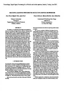
wheel and accelerator pedal position and motion, the test vehicle speed variation, lane maintenance and carfollowing distance. Based on the results of previous work (2,3). only steering wheel data were used to develop the fatigue detection algorithm. Lane maintenance data were used for further evaluation. Scoring Steering Performance Steering wheel position was analyzed in the time, frequency and phase domains. Scoring functions were devised in each domain to quantify different types of steering behavior. Time-Based Functions - From the graph of steering wheel angle versus time (Figure 1) or steering wheel angular velocity versus time, differences in the steering

874

15 /

I

-15 1 800 15

-15

816

832

848

,

864 I

1

I

6412

6444

6428

6460

6476

Figure 1. Early and late steering behavior in the time domain for Driver 8 (3).

Loose loops, occasionally straying far from the origin, indicated longer-duration feedback, and also indicated that the driver was relying on larger and coarser steering wheel movements to control his vehicle. It was hypothesized that this behavior indicated the driver was fatigued. Small sub-clusters on the horizontal axis away from the origin (large steering angle but no angular velocity) were indicative of cornering and were particularly inappropriate on straight legs. A sample of this behavior can be seen between +5 and +lO degrees on the O-axis of the Late Night phase plot in Figure 4. Weighting functions that quantified and penalized loose loops and small sub-clusters on the e-axis were developed. co Early Night

loo

15

-15

-100

d

0.5

1 Late Night

Frequency (Hz)

qoo

0

Figure 2. Variations in the power spectrum of steering wheel angle for Driver 6 (3). 8

,\

15

-15

-100

Figure 4. Sample Phase Plots from Driver 8 Showing Steering Behavior and Control Ellipse of -7.5 5 0 2 7.5” and -50 < o 5 50 ‘Is. 0

1

2

3

4

A subset of the phase-basedweighting functions made use of a control ellipse. It was hypothesized that there was an area of the phase plot surrounding the origin in which alert drivers remained. Based on the phase plot

Frequency (Hz)

Figure 3. Variations in the power spectrum of steering wheel angular velocity for Driver 6 (3).

875

shape of a number of early night legs from a number of drivers. a preliminary ellipse shape was chosen with a horizontal axis (steer angle, S) of 15 degrees (from -7.5” to -7.5”) and vertical axis (steer angular velocity, o) of 100 degrees/second (from -50 “is to +50 “is). Weighting functions that incorporated only portions of the phase plot outside the acceptable control ellipse were devised. ALGORITHM

halfway between “Moderately Drowsy” and “Very Drowsy” on the SED continuum (6). RESULTS Based on SED levels of 80 to 100, cutoff limits (Table 2) for each weighting function were determined from the graphs in Figure 5. The lower end of the ranges in Table 2 resulted from the inclusion of all drivers and a SED cutoff level of SO. Four drivers (3, 8, 13, and IS) were found to significantly alter the average SED and a similar series of graphs excluding these drivers was also examined (Figure 5). Three of these four drivers (3, 8, and 15) reached the maximum SED level (“Extremely Drowsy”) within 30 legs (10 laps) of the start of the test. Both Drivers 3 and 15 reached a SED level of 100 within 10 legs of the start of the test. Driver 8 reached a SED level of 100 about 22 legs into his test, and fell asleep on leg 75. For drivers 3, 8, and 15, the steering-based weighting functions lagged the rise in SED. Because of this lag and the rapid rise in SED, the three weighting functions did not reach their cutoff limits until maximum SED had been reached. It was hypothesized that in the real world the transition to “Extremely Drowsy” would not often occur this rapidly and therefore weighting-function cutoff limits excluding these data were also examined.

DEVELOPMENT

As reported earlier (6), SED is a comprehensive measure of driver fatigue. SED was therefore used as the reference in the development of an algorithm to determine when a driver became fatigued. To identify which weighting functions correlated best with fatigue, the coefficient of determination (r’) between the rank order (Spearman) of each weighting function and SED was calculated. The mean r2 across all drivers was then calculated. A minimum useful coefficient of determination was arbitrarily set to 0.5. As determined previously, ten weighting functions met this criterion (3). Of the ten, three functions were selected for the algorithm: Amp-D2-Theta, Wt Flat 0, and Outside (%) (Appendix A). The former two functions were selected because they correlated most strongly with SED. These two functions represented time-based and phase-based (control ellipse independent) measures. Of 7 phase-based measures which relied on the control ellipse, Outside (%) was selected because it correlated well with drivers who did not correlate well with the first two functions. Together, these three functions correlated with 15 of the 17 drivers, Only Drivers 3 and 4 did not correlate with these or any other functions. The 6-leg averaged value of the three functions was calculated simultaneously from the fourth leg of each driver’s test (the results from the first three legs were ignored). A simple algorithm that monitored the value of these three functions until one exceeded a specific value was used. These specific values (termed the cutoff limits) were determined by independently plotting the average SED value of all drivers over a range of possible cutoff limits (Figure 5). To select cutoff limits for each function, some level of fatigue must be used as a threshold above which a driver is deemed to be too tired to drive. The setting of this threshold level is outside the scope of this study. In order to develop a working algorithm, a SED range between 80 and 100 was arbitrarily used as the threshold above which a driver was too tired to continue driving. A SED score of 80 represents a “Moderately Drowsy” level and a score of 100 represents the level

Table 2. Proposed Cutoffs for Steering-Based

Functions

The upper cutoff limits in Table 2 resulted from the exclusion of Drivers 3, 8, 13, and 15 and a SED cutoff level of 100. Both the upper limits and lower limits of the ranges proposed in Table 2 were applied to the present data set of 17 drivers. The results are given in Appendix B. The upper limit of Outside (%) was assessed in greater detail. due to the relatively flat slope between SED values of 80 and 100 (Figure 5). An SED value of 100 corresponded to a Outside (%) value of 10, whereas a SED value of 93 corresponded to an Outside (%) value of about 6. Using an upper limit of 10 for Outside (%), only two drivers were captured (2 and 11). Decreasing the upper cutoff limit to 6 resulted in nine drivers being captured (1, 2, 3, 6, 9: 11, 12, 15 and 18).

876

Table 3 shows the average, minimum and maximum SED levels across all drivers for the upper and lower bounds of the proposed cutoff limits. Using the lower cutoff limits, all but four drivers were trapped before their SED level reached 100

1

I

(“Moderately to Very Drowsy”). Five drivers were caught before their SED level reached 40 (“Slightly Drowsy”).

Table 3. SED at Cutoff Limits Cutoff Limits / Average SED Lower / 68 (12 - 127) 96 (39 - 152)

1

Upper

Using the upper cutoff limits, eight drivers reached a SED level greater than 100. three of which were at about 150 when trapped. Only one driver was trapped before his SED level reached 40, but six were trapped before their SED level reached X0 (“Moderately Drowsy”).

x77

A comparison of the algorithm-predicted cutoff points with the lane breach data is shown in Figure 6. The horizontal axis of Figure 6, labeled “Legs”, is the number of 6-leg averages. For instance, leg 20 on the horizontal axis corresponds to the average of legs 20 through 25.

DISCUSSION The current algorithm and cutoff limits show that a fatigue detection algorithm based on steering wheel motion can be constructed. The algorithm trapped all 17 drivers before the end of their night drive. Figure 6 shows that for twelve of the 17 drivers, the algorithm predicted driver fatigue before or at the same time as the first lane breach occurred. For the remaining five drivers, the first lane breach and the first lane breach greater than 1 second occurred before the lower cutoff limit of the algorithm detected driver fatigue. For three of these five drivers (4, 7, and lo), the algorithm predicted fatigue before a lane breach greater than 15 cm occurred. Also, for three others among the same five drivers (6, 10, and 1S), the lower limit of the algorithm detected fatigue within 5 legs of the first lane breach, i.e., within the period of the running average interval. In only two of the five late-detection cases did a lane breach precede detection by more than 5 legs (Drivers 4 and 12). For both drivers however, the algorithm predicted fatigue before their first lane breach greater than 15 cm. Further examination of Driver 4’s lane breach data indicated that his next lane breach (after the one shown at Leg 12) occurred at Leg 56 on this graph above the lower cutoff limit of the algorithm. Driver 12’s next lane breach, on the other hand, occurred at Leg 12 on this graph - still about 8 legs below the lower cutoff limit of the algorithm. Only two drivers (6 and 18) were not captured by the algorithm before a lane breach of 15 cm. In both cases, the algorithm detected fatigue within five legs of the start of the test and within two legs of the breach. The algorithm failure for Driver 6 may be related to his initial elevated level of drowsiness. His test was interrupted twice by electrical failures and the start of his driving data was preceded by about one hour of lost data. Driver 18’s early lane breaches were a result of extended pre-comer maneuvers (he breached the lane for 8 seconds prior to one comer). It was not until leg 12 near the upper end of the algorithm-predicted range - that he breached the lane at a distance from the comer. The average driver reached the lower cutoff limit at Leg 12 and the upper cutoff limit at leg 36. Excluding Drivers 4 and 7, both of whom had long cutoff intervals, the average upper cutoff limit was reached at leg 24. If lane breach is a valid indicator of driver fatigue, then the results depicted in Figure 6 suggest that the lower cutoff limits proposed in Table 2 may be slightly high for some drivers. For other drivers, even the upper cutoff limit was low. Driver 13 was the only driver who did not reach a SED level of 100 - his maximum SED tias 9 1. He was the driver who received the largest portion of his normal sleep in the 48 hours preceding the test (96 percent). His gradual increase in SED may be more indicative of a real-

. i:

* / .

‘1

+

2

* + .

3

I

. +

:/

I

I +

;

Leq

+

I

c ‘t-.-----i-

25

4c

P

si

8:

“X --

Figure 6. Summary of Algorithm Cutoff Legs.

:i3

‘L:

5c

vi---

and Lane Breach

In Figure 6, the thin horizontal line terminated by the vertical mark represents the total number of 6-leg averages for each driver. This value is 5 less than the number of legs shown in Table 1 because of the effect of averaging 6 legs. The thicker portion of the line represents the range of cutoff points predicted by the algorithm using the lower and upper cutoff limits in Table 2. The lower cutoff limit corresponds to the left end of the thick line and the upper cutoff limit corresponds to the right end of the thick line. The three symbols (0, o, and +) depict the points when the first lane breach occurred (*), the first lane breach greater than 15 cm occurred (o), and the first lane breach greater than 1 second in duration occurred (+). If a symbol is absent, then a lane breach meeting its criterion did not occur. To minimize the effect of comer-induced lane breaches, only lane breaches more than 4 seconds from the comer are shown. The relative position of the lane breach data to the thick horizontal line for each driver shows the effectiveness of the algorithm and cutoff limits.

878

maintenance and steering wheel data will reduce the potential for misdiagnosing driver fatigue. In summary, three steering-based weighting functions are recommended for detecting driver fatigue: Outside (%), Wt Flat 0, and Amp-D2-Theta. The proposed absolute cutoff limits for the three weighting functions are shown in Table 2. These proposed cutoff limits were based on SED levels of 80 and 100, and on data acquired under controlled conditions. They are necessarily preliminary and are subject to confirmation by on-theroad testing. The proposed algorithm captured all 17 drivers before the end of their night test. Twelve of the drivers were detected before any lane breaches occurred. Only two drivers were not captured before a lane breach greater than 15 cm occurred, and both of these drivers were captured within two legs of this lane breach.

world driver and suggests that cutoffs based on a SED between 80 and 100 are too high. This gradual increase in drowsiness of drivers not sleep-deprived should be explored further. An optimal value for each cutoff limit has not been chosen for two reasons: first, data gathered at highway speeds with drivers who are initially alert and grow drowsy will be required to properly set the cutoff limits; and second, a decision on what level of SED constitutes a dangerous level must be addressed and resolved. In addition, the question of absolute cutoff limits (applicable to all drivers) or relative cutoff limits (individual driver specific limits) has not been explored. To properly determine relative cutoff limits (e.g. doubling of a weighting function within a specific time interval), the alert values for the three weighting functions must be known. These data were not available for the drivers in this study. The weighting functions and algorithms were developed from data gathered in straight leg sections with intervening comers. On average, half of each lap was spent cornering and the other half was spent on the straight sections, which means that only half of the data gathered was used. In a real world application, data would probably be gathered more continuously and the time length of the running averages may need modification. It is not known to what degree the intervening comers delayed fatigue development. Data gathered from truck drivers on the road will be required to confirm the appropriate time length for the running averages. The cutoff values were developed from data gathered from a specific truck on a specific track under test conditions. Moreover, all of the data were gathered at a nominal speed of 42 km/h. Testing of other trucks on real roads at highway speeds must be conducted to validate the weighting functions, the algorithm, and the cutoff limits. Different steering-box ratios on other trucks may also alter the cutoff limits. If a fatigue detection device is to be used predominantly on highways, then some means of determining that the vehicle is travelling at highway speed will be necessary. For example, the frequency of gear shifts could be monitored. Periods of high-speed travel and low gear-shifting frequency could be useful precursors to the onset of fatigue (7). Almost all of the drivers in this study were sleep-deprived prior to starting their test. Because the drivers were not monitored from an alert condition into a fatigued condition while driving, the proposed cutoff limits may be subject to modification. Real-world testing of initially-alert drivers must be conducted to confirm or modify these cutoff limits. Lane maintenance may be a valuable independent measure of driver fatigue as imaging technology develops and becomes more affordable. Combining lane

ACKNOWLEDGMENTS The data for this paper were collected for a fatigued driver identification study for the Insurance Corporation of British Columbia (ICBC). The authors would like to thank ICBC for permitting the publication of these findings. REFERENCES 1. Knipling, RA., and Wang, J-S, “Crashes and Fatalities Related to Driver Drowsiness/Fatigue”, Research note, Washington, DC, U.S. Department of Transportation, NHTSA, 1994. 2. Siegmund, GP, King, DJ, and Mumford, DK, “Correlation of Heavy-Truck Driver Fatigue with Vehicle-Based Control Measures”, SAE 952594, 1995. 3. Siegmund, GP, King, DJ, and Mumford, DK, “Correlation of Steering Behavior with HeavyTruck Driver Fatigue”, SAE 961683, 1996. 4. King, DJ, Siegmund, GP and Montgomery, DT, “Outfitting a Freightliner Tractor for Measuring Driver Fatigue and Vehicle Kinematics During Closed-Track Testing”, SAE 942326, 1994. 5. Ellsworth, LA, Wreggit, SS, and Wierwille, WW, “Research on Vehicle-Based Driver Status/Performance Monitoring”; Third Semi-Annual Research Report, Sept. 92 to Mar 93. Dept. of Industrial and Systems Engineering, Report No. 93-02, Blacksburg Virginia: Virginia Polytechnic Institute and State University; 1993. 6. Wierwille WW and Ellsworth LA. “Evaluation of Driver Drowsiness by Trained Raters”, Accident Analysis and Prevention, Vol. 26, No. 5, pp. 571581,1994. 7. Yamamoto K, Hirata Y, and Higuchi S, “Estimate of Driver’s Alertness Level Using Fuzzy Method”, SAE 942321. 1994.

879

APPENDIX FUNCTION

A - STEERING-BASED FORMULAE

WEIGHTING Phase-Based Weighting Functions

Various weighting functions based on steering angle (0), steering angular velocity (o), and combinations of the two were developed. Three ways of viewing the data were used to develop the weighting functions: Time-based: weighting functions developed from variations in 8 or o plotted against time, Frequency-based: weighting functions developed from variations in the power spectrum, Phase-based: weighting functions developed from variations in 8 plotted against w (no time dependence).

Phase-based weighting functions were developed by examining the phase plot of steering angle (0) versus steering angular velocity (w) (see Figure A2). These functions were broken into two sub-groups: functions dependent on a hypothesized control ellipse, and functions independent of the control ellipse. co 100 -

8

The three weighting functions referred to in this paper are outlined below: Time-Based Weighting Functions

-1

Both 8 and w were plotted against time and weighting functions were devised to score variations present in these variables as the driver tired. As discussed, AmppD2-Theta was selected for determining a cutoff point: Amplitude Duration Squared Theta - (Amp-D2-Theta) - Each distinct area between theta and the mean of theta over the length of one leg was multiplied by the length of time the steering angle remained on that side of the mean. The area under the O-curve was calculated using trapezoidal integration. Figure Al shows the variables used to calculate AmppD2-Theta.

5

-100

i

Figure A2. Example of Phase Plot with Control Ellipse. Ellipse-Dependent Weighting Functions A control ellipse with a horizontal (Cl) axis length of

2a and a vertical (0) axis length of 2b was superimposed onto the phase plot of 8 versus o. Steering behavior outside the control ellipse was penalized, whereas steering behavior inside the ellipse was considered normal. Different ellipse dimensions (a,b) were also investigated: a was varied between 3” and 9” in 1.5” increments, and b was varied between 2O”is and 6O”is in 1O”/s increments. Values of f7.Y and f50”/s were selected.

where A; = thejth area block in the (EM,) data of the leg, ‘- the length of thejth area block in the leg, ;‘L the total number of area blocks in the leg, = Z+l (see Zero Crossings below), N = total number of samples in leg, and 100 is a scaling factor. 4(68-1 3 A(-)

Outside (%) - (Outside) - The percentage of (8,w) points per leg outside the control ellipse including single point episodes. Outside = 100 G 642) N

where n = number of points outside control ellipse, N = total number of sampled points in leg, and 100 is a scaling factor.

Ellipse-Independent I 4’ Figure Al.

Weighting Functions

Weight Flat Zero - (Wt Flat 0) - only (@,vi) points in the phase space satisfying the condition / w ( C:o, with, o, = 5 O/sare included in the calculation. All points

Definition of variables for calculating Amp-DZ-Theta.

satisfying this condition

distance from the origin.

880

are weighted by the square of the

(43)

only for I0; I 5 W, where f$ = ith value of the steerangle, 8,= mean value of all 8’s for leg, a = half axis length of ellipse in 0 dimension, Oi = ith value of steerangular velocity, w, = cutoff value of omega(5 O/s), N = total number of sampledpoints in leg, and 100 is a scaling factor. APPENDIX

B - ALGORITHM

PERFORMANCE

Two tables are presented, showing the results of running the algorithm through the current set of 17 drivers using first the lower cutoff limits (Table Bl) and then the upper cutoff limits (Table B2).

881

ALGORITHM Table Bl

RESULTS

Cutoff results for all Drivers using a SED value of 80

Total legs driven

1

2

3

4

6

7

8

99

78

102

144

39

156

75

Cutoff Leg

Driver Number 9 10 11

12

13

14

15

16

18

19

Min

Avg

Max

93

96

120

135

35

69

117

108

35

99

156

93

120

4

3

8

35

3

3

21

23

7

12

20

3

3

4

18

3

27

3

12

35

Leg where SED = 80

17

16

1

74

2

128

10

30

3

21

21

106

47

2

15

88

28

1

36

128

SED at cutoff

39

54

122

67

86

18

127

69

109

60

79

12

35

92

103

19

75

12

68

127

124

150

157

132

135

103

160

135

141

154

153

91

137

160

155

151

154

91

141

160

39

54

122

73

86

18

127

69

109

60

79

12

35

92

103

19

75

12

69

127

Maximum SED for all legs Maximum SED before capture

Wt Flat 0 Amp-D2-Theta

Table 82 Cutoff results for all Drivers using a SED value of 100

Total legs driven Cutoff Leg

Driver Number 9 10 11

1

2

3

4

6

7

8

99

78

102

144

39

156

75

93

93

120

12

13

14

15

16

18

19

Min

Avg

Max

96

120

135

35

69

117

108

35

98.8

156

7

3

24

128

3

117

44

40

23

24

34

47

30

15

22

12

32

3

35.6

128

Leg where SED = 100

23

21

4

102

7

143

14

51

6

46

28

999

73

6

18

94

32

4

98

999

SED at cutoff

44

54

151

123

86

68

153

95

131

89

116

43

70

149

123

38

101

38

96

153

124

150

157

132

135

103

160

135

141

154

153

91

137

160

155

151

154

91

141

160

44

54

151

132

86

69

158

95

131

89

116

43

70

149

123

38

101

38

97

158

Maximum SED for all legs Maximum SED before capture

Amp-D2-Theta