An association algorithm for tracking multiple moving objects Yann Lemeret, Eric Lefevre and Daniel Jolly
Abstract— In the field of intelligent vehicle and in order to raise the road safety, we are trying to improve the driver’s assistance and more particularly obstacles detection systems. The objects are detected with sensors laid out on a car, and then, they are tracked with an association algorithm. We have modified M. Rombaut association algorithm in order to have a better decision when the data reliability decrease or if one sensor fails. This paper presents M. Rombaut association algorithm and the modification we have made on it. Then, a comparison between the two association algorithms for a decreasing data reliability is made thanks to simulated data. Finally we have tested the robustness of the two algorithms with data coming from a CCD camera.
I. I NTRODUCTION Our laboratory is integrated into a Federative Structure named GRAISyHM (Groupement de Recherche en Automatisation Intégrée et Système Homme Machine du Nord Pas de Calais). Its aim is to structure and develop the research in Automatics in all the laboratories in the region Nord Pas de Calais. We are currently working on the project RaViOLi (Radar Vision Orientable et Lidar). This is a regional project dedicated to long range detection and tracking of obstacles. It is based on data fusion, using the Evidence theory, of a stereovision system, a radar and a lidar. There are also some European projects that are working on driver’s assistance in order to raise the road safety : Carsense, Prométheus [1], Argo . . . . This paper deals with the modification of M. Rombaut tracking algorithm in order to improve tracking of objects detected by various sensors when the data reliability decrease or if the system has to work with only one sensor. A comparison is made between the two algorithms using synthetic and real data. The fusion we use in this algorithm is made thanks to the Evidence theory. This paper will not present this theory as there are many paper that already describe it like [2], [3], [4], [5]. In section II, we describe the method for the masses creation. Then, section III shows M. Rombaut association algorithm and the modification we have made on it. Finally, the results we obtain for both algorithms, for simulated and real data, are in section IV. Y. Lemeret is with LGI2A, Faculté des Sciences Appliquées, Université d’Artois, rue de l’université, Technoparc Futura, 62400 Béthune, France
[email protected]
E. Lefevre is with LGI2A, Faculté des Sciences Appliquées, Université d’Artois, rue de l’université, Technoparc Futura, 62400 Béthune, France
[email protected]
D. Jolly is with LGI2A, Faculté des Sciences Appliquées, Université d’Artois, rue de l’université, Technoparc Futura, 62400 Béthune, France
[email protected]
II. C REATION OF MASSES In case of an intelligent vehicle, objects are detected by means of sensors laid out on a vehicle. From these sensors that are used for RaViOLi, we know the kind of information we will have to work with which is expressed in (distance;angle) : (ρ; Θ). In addition, we also know the dimensions of the object. The aim is to follow vehicles. Therefore, we must be able to find them from one moment to another. We use all the information we have to create several masses sets indicating the relations that exist between perceived objects at time t and those known from time t − 1. We will note Xi the Perceived objects (i = 1 : N bP ) at time t by the sensors and Yj the Known objects (j = 1 : N bK). The known objects are perceived objects from the previous sample time that were stored in a memory. In a first time, we have to define the frame of discernment on which we will work. We have chosen two hypotheses : Ω = {(Xi RYj ); (Xi RYj )}. Either the perceived object is the same as the known one (in relation : (Xi RYj )), or it is not (not in relation : (Xi RYj )) [6]. The first step consists in creating belief functions using the information. We build a different masses set for each usable information of each sensor. Mathematical equations of the masses set, that allow to determine whether objects are in relation or not, is based on a negative exponential introduced by Denoeux [7] : 2
m(Xi RYj ) = α0 · exp(−ei,j ) 2 m(Xi RYj ) = α0 · (1 − exp(−ei,j ) ) m(Ωi,j ) = 1 − α0
(1)
with ei,j the variation between two informations (distances, angles, or speed) from perceived objects Xi and known Yj . α0 is a coefficient that characterizes the sensor reliability. There is then one masses set for the distance (Fig. 1) and one for the angle for each sensor. Next step consists in combining masses set of distance and angle for each sensor, and then to combine between the various sensors. To make the data fusion, we use the evidence theory with the conjonctive operator from Dempster and normalisation. At the end of those two fusion steps, we get as masses set as the number of possible relation between objects. Now we have to decide which are the recognized objects, those that appeared and those that disappeared. That is what is described in the next section.
Fig. 1. Computation of relation masses for known and perceived using the variation of distances between them.
III. O BJECTS ASSOCIATION Taking the decision when associating objects is done thanks to a fusion algorithm which was developed by M. Rombaut [8]. This algorithm was improved by D. Gruyer [9]. A. Mathematical formulation The algorithm is based on the calculation of some masses. We compute the relation masses for a given object i to all the objects j. These masses are noted mi,. . We proceed next to the operation that consists in computing the relation masses of each object j to all other i. These masses are noted m.,j . The mathematical formulation adopted for mi,. and the m.,j are :
We can notice that the non relation masses are not computed. However, these informations are not necessary for the decision : deciding that Xi is not in relation with Yj does not give any information about the other associations. We can also see two new hypotheses mi,. (Xi R∗) and m.,j (Yj R∗). In these hypotheses, ∗ represents the fact that one object is in relation with none of the other. Thus if a perceived object Xi is not associated, it is a new object and if a known object is not associated, it has disappeared (masked by another object, out of range, ...). The decision is taken according to the two masses set mi,. and m.,j . We choose the couples that have the maximum of credibility in the two masses set. B. New formulation When using those equations [10], we have discovered that in some situations, they were not working well. Indeed, the masses mi,j (Xi RYj ), are added on mi,. (Ωi,. ) and m.,j (Ω.,j ). If it does not matter for the decision because deciding that Xi is not in relation with Yj does not give any information about the good relation, the way in which the formulas are made adds these masses on Ω and can lead to choose a bad decision. For example with one perceived and two known giving the following masses sets : m1,1 (X1 RY1 ) = 0.2 m1,1 (X1 RY1 ) = 0.45 m1,1 (Ω1,1 ) = 0.35
m1,2 (X1 RY2 ) = 0.45 m1,2 (X1 RY2 ) = 0.15 m1,2 (Ω1,2 ) = 0.4
We have :
Mi,.
Y1 = Y2 ∗ Ω1,.
M.,j = Y1 Y2
X1 0.2 0.45
X1 0.121 0.396 0.073 0.41
∗ 0.45 0.15
Ω.,j 0.35 0.4
From the first matrix (mi,. ), we can deduce that we do not know the relation on X1 : m1,. (Ω1,. ) = 0.41 while seeing that m1,. (X1 RY2 ) = 0.396. From the second matrix, we can decide that Y1 disappears and that X1 is in relation with Y2 . So there is a problem to decide the couples. To solve it, we have decided to modify the equations that compute the masses mi,. and m.,j . This modification consists in increasing the masses of relation (Xi RYj ) and the mass on star with the non relation masses (Xi RYk )(k6=j) that do not contradict the relation hypothesis. The new mi,. and the m.,j are defined like this :
the product (m1,1 (X1 RY1 ) · m1,2 (Ω1,2 ) · m1,3 (Ω1,3 )), we cannot decide where the mass should go, so we put 13 to the first relation (m1,. (X1 RY2 )), 31 to the second (m1,. (X1 RY3 )) and 31 to the mass on star (m1,. (X1 R∗)), and so on till we divide by N bK (or N bP ). Considering again the example, we have : X1 Y1 0.15 0.495 Mi,. = Y2 ∗ 0.201 Ω1,. 0.154
M.,j = Y1 Y2
X1 0.2 0.45
∗ 0.45 0.15
Ω.,j 0.35 0.4
This time, there is no ambiguity about the best decision which is : (X1 RY2 ) and Y1 disappears. Next section shows a comparison between the two formulas using synthetic and real data. IV. E XPERIMENTAL RESULTS The aim of this part is to validate the association formulas we have made thanks to results obtained from simulated or real data. The first part illustrates the use of the formulas(1) with synthetic data and a decreasing data reliability. The second part shows the results with real data. A. Synthetic data
In the terms of relation and star, coefficients appear : ( N 1bK , . . . , 21 ) for mi,. and ( N1bP , . . . , 12 ) for m.,j . They correspond to an equal distribution of the mass when there are one or more masses on Ω multiplied with the non relation masses. Indeed, with one perceived object and two known, if we multiply m1,2 (X1 RY2 ) by m1,1 (Ω1,1 ), it means that we are sure that X1 is not in relation with Y2 , so as the framework is exhaustive and closed, the result goes on m1,. (X1 RY1 ) and m1,. (X1 R∗) (multiplied by 12 ). In case of three known objects, if we have two masses on Ω in
We have taken two objects side by side with the same speed and distant from 1m from each other. Those two vehicles move away progressively from the sensor (from 20 to 100m with a constant speed of 5m.s−1 ) which leads to the fall of the reliability coefficient (from 0.9 at 20m to 0.3 at 100m). Fig. 2 represents the evolution of the decision reliability in function of the sensor reliability for M. Rombaut’s algorithm and the one we presented. We consider that the decision is not completely reliable when the variation between the mass of good decision and another one is lower than a threshold we have set to 0.1 in this case. When the reliability is greater than 0.69, the two algorithms give the same results. However, our algorithm is able to give a reliable decision till a data reliability of 0.49. For M. Rombaut algorithm, the decision is not reliable below 0.69 and is false if the data reliability falls below 0.63. We have tested with many threshold values and we have always arrived at the same conclusion : our algorithm is better when the reliability decreases. When real tests could be made, it would be interesting to plot the percentage of good decisions of the two algorithms with various reliability from several scenarii. Fig. 3 shows the evolution of the non specificity in function of the data reliability. As we can see, our formulas 1 In order to make easier the computational stage, in this part, i ranges from 0 to N bP − 1, and j from 0 to N bK − 1
gravity center in the image. So we have information (ρ, Θ), for two different sensors(2) [11]. As we are not specialized in image processing, the measures we have extracted were very noisy. Indeed, at 70m, we can have for the same object from an image to the next a variation of 20m. In angle, it can reach 0.02rd for a measure of 0.01rd. First, we have extracted the measures from only one sensor of one object. This object is followed during 260 images (almost 10s) and is located at almost 70m from the sensor. Figure (Fig. 4) shows the evolution of the data reliability for the perceived object.
1 M. Rombaut formulas Modified formulas 0.9
0.8
Decision reliability
0.7
0.6
0.5
0.4
0.3
0.2
0.1
0.65 0 0.3
0.4
0.5
0.6 Data reliability
0.7
0.8
0.9
0.6
Fig. 2. Evolution of the decision reliability in function of the data reliability. 0.55 1.4 M. Rombaut formulas Modified formulas
Reliability
0.5
1.2
0.45
Non Specificity
1
0.4
0.8
0.35
0.6
0.3
0.4
0.25
0.2
50
Fig. 4.
0 0.3
Fig. 3.
0
0.4
0.5
0.6 Data reliability
0.7
0.8
0.9
Evolution of the non specificity in function of the reliability.
give more specific masses set, so there is less uncertainty on the best decision. B. Real data In order to improve the association algorithm and to test it robustness, we have decided to use real data. These data come from a simple DV camera that we have placed behind the windshield of a car. This DV camera has a CCD sensor. The resolution is 720x576 pixels, the angle ranges from −0.5 to +0.5 radians (almost ±30◦ ) and works at 25 images per seconde (∆t = 0.04s). For the calibration, we have filmed a sequence on a parking lot where there was a reference car parked. A pocket laser telemeter allows us to measure the distance between the camera and the car. The measures were done from 0 to 60m, because after, it was difficult to point the laser on the car. From the calibration sequence, while supposing that detected objects are cars, we have computed by two different interpolation methods two equations that give the distance in function of the object height and width in the image. The angle is extracted from the position of the
100
150 Number of images
200
250
300
Evolution of the data reliability.
We have plotted the comparison between the two association algorithms for the M0,. (Fig. 5), the M.,0 (Fig. 6) and the global decision using the those two informations (Fig. 7). In Fig. 5 and 6, we can see that with the new formulas, we always have the relation mass ((X0 RY0 ) and (Y0 RX0 )) and the mass on star ((X0 R∗) and (Y0 R∗)) equal or higher than with M.Rombaut formulas. With the new formulas, the mass on Ω is always under the mass we obtain with M. Rombaut formulas. So the decisions on M0,. and M.,0 are different for the two algorithms. Thus, the global decisions (Fig. 7) are different too. With our algorithm, we do not have any decision on Ω, so we can always decide. Instead, we have more decisions on ∗ which is not a problem because even if we decide that the perceived object is a new object (tracking is lost), the object is detected. Whereas deciding Ω involves that we do not have any information about the object (maybe it does not exist). Now, we have extracted the measures of one object (the same object as in the previous section) from the two sensors (Sec. IV-B). The data reliability for this object has already been plotted (Fig. 4). The comparison between the two association algorithms for the M0,. is plotted in Fig. 8 and Fig. 9 for the M.,0 . The 2 The fact that we have used two different interpolation methods leads us to two sources of information. So we can say that we have two sensors.
M (X R Y ) 0,.
0
0
Mass
1
M. Rombaut formulas Modified formulas
0.5
0
0
50
100
150 M0,.(X0 R *)
200
Mass
1
300
M. Rombaut formulas Modified formulas
0.5
0
0
50
100
150 M0,.(Ω0,.)
200
1 Mass
250
250
300
M. Rombaut formulas Modified formulas
global decision using the those two informations is plotted in Fig. 10. In Fig. 8 and 9, we can see that with the new formulas, we always have the relation mass ((X0 RY0 ) and (Y0 RX0 )) and the mass on star ((X0 R∗) and (Y0 R∗)) equal or higher than with M. Rombaut formulas but this time, thanks to the sensor fusion, there is less variation between the two algorithms. With the new formulas, the mass on Ω is still under the mass we obtain with M. Rombaut formulas but once again, the variation is less than with one sensor. In order to test the robustness of our algorithm, between images 175 and 225, one sensor fails. During this time, we can see that our algorithm is still working fine.
0.5 M (X R Y ) 0,.
0
50
100
150 Number of images
200
250
0
0
1
300 Mass
0
Fig. 5. Evolution of the mass of relation, star and Ω for the M0,. with one perceived object.
0.5
0
M.,0(Y0 R X0)
M. Rombaut formulas Modified formulas
0
50
100
150 M0,.(X0 R *)
200
1 Mass
Mass
0.5
0.5 0 0
0
50
100
150 M.,0(Y0 R *)
200
250
0
50
100
150 M0,.(Ω0,.)
200
1
Mass
Mass
M. Rombaut formulas Modified formulas
0.6
250
300
300 M. Rombaut formulas Modified formulas
0.8 0.5
0.4 0
0.2
0 0
0
50
100
150 M.,0(Ω.,0)
200
250
50
100
300
1
150 Number of images
200
250
300
Fig. 8. Evolution of the mass of relation, star and Ω for the M0,. with one perceived object.
M. Rombaut formulas Modified formulas Mass
300
M. Rombaut formulas Modified formulas
1 M. Rombaut formulas Modified formulas
250
0.5
0
0
50
100
150 Number of images
200
250
300
M.,0(Y0 R X0)
Fig. 6. Evolution of the mass of relation, star and Ω for the M.,0 with one perceived object.
Mass
1
M. Rombaut formulas Modified formulas
0.5
0
0
50
100
150 M.,0(Y0 R *)
200
Mass
1
300
M. Rombaut formulas Modified formulas
0.5
0
0
50
100
150 M.,0(Ω.,0)
200
1 Mass
250
250
300
M. Rombaut formulas Modified formulas
0.5
0 0
50
100
150
200
250
300
Fig. 9. Evolution of the mass of relation, star and Ω for the M.,0 with one perceived object.
Fig. 7. Comparison of the global decision (using M0,. and M.,0 ) on association for the two algorithms. Decision plotted in the bottom corresponds to M. Rombaut algorithm and in the upper for the Modified formulas.
This is confirmed with the global decision (Fig. 10). The decisions are not very different when the two sensors operate. But, when one sensor fails (between 175 and 225), we can see that our algorithm still track the objet most of time. When it is not tracked, our algorithm decide that it is a new
object (mass on star) so that is not a real problem. Whereas with M. Rombaut algorithm we have a lot of decision on Ω and that involves we do not have any information about the object.
Fig. 10. Comparison of the global decision (using M0,. and M.,0 ) on association for the two algorithms. Decision plotted in the bottom corresponds to M. Rombaut algorithm and in the upper for the Modified formulas.
V. C ONCLUSION AND FUTURE WORK We have presented in this article an improvement of an association algorithm. This algorithm is used to track moving vehicles. We have changed the distribution of mass between the hypotheses in order to reduce the number of ambiguous and bad decisions. This algorithm was tested on synthetic and real noisy data. We obtain better results with the modified formulas especially when the reliability is weak and when there is only one sensor working. We have reduced the number of non decisions and made easier the choice of the good decision while increasing the gap between the mass for the best hypothesis and the others. We can still improve the detection and tracking of objects while adding to this algorithm a predicting filter [12], [13], [14]. We can thus predict future associations. This information could be used to confirm at this time the associations that are made or to reduce the ambiguous decisions on some associations. It can also be used as a new sensor that we can put in the stage of data fusion. R EFERENCES [1] B. Dryselins, J. Broughton, L. Ekman, C. Hyden, G. Malaterre, S. Petica, R. Risser, and P. Van El Slande. Traffic safety in prometheus. Technical report, INRETS, Avril 1994. [2] A. Dempster. Upper and lower probabilities induced by multivalued mapping. Annals of Mathematical Statistics, AMS-38:325–339, 1967. [3] G. Shafer. A Mathematical Theory of Evidence. Princeton University Press, Princeton, New Jersey, 1976. [4] P. Smets. What is dempster-shafer’s model ? In R.R. Yager, M. Fedrizzi, and J. Kacprzyk, editors, Advances in the DempsterShafer Theory of Evidence, pages 5–34. Wiley, 1994. [5] P. Smets and R. Kennes. The transferable belief model. Artificial Intelligence, 66(2):191–234, 1994.
[6] M. Rombaut and V. Cherfaoui. Decision making in data fusion using dempster-shafer’s theory. In 3th IFAC Symposium on Intelligent Components and Instrumentation for Control Applications, Annecy, France, 9-11 Juin 1997. [7] T. Denoeux. A k-nearest neighbour classification rule based on dempster-shafer theory. IEEE Transactions on Systems, Man and Cybernetics, 25(5):804–813, 1995. [8] M. Rombaut. Decision in multi-obstacle matching process using the theory of belief. In AVCS’98, pages 63–68, 1998. [9] D.Gruyer, C.Royère, and V. Cherfaoui. Credibilist multi-sensors fusion for the mapping of dynamic environnement. In Thrid International Conference on Information Fusion (FUSION’2000), page TuC2, 2000. [10] Y. Lemeret, E. Lefevre, and D. Jolly. Detection and tracking of moving objects. In IEEE sponsored international conference on Artificial Intelligence Systems (AIS), September 2005. [11] Y. Lemeret, E. Lefevre, and D. Jolly. Tracking cars and prediction of their trajectories. In IEEE sponsored International Conference on Machine Intelligence (ACIDCA-ICMI), pages 64–69, November 2005. [12] R. Bucy. Non linear filtering. IEEE Transaction on Automatic Control, 10, 1965. [13] S.J Julier and J.K Uhlmann. A new extension of the kalman filter to nonlinear systems. SPIE AeroSense Symposium, 21-24 April 1997. [14] J.C Noyer, P. Lanvin, and M. Benjelloun. Non-linear matched filtering for object detection and tracking. Pattern Recognition Letters, 25:655– 668, 2004.