sequences using Lowe's Scale-Invariant Feature Transform. (SIFT) [1, 9]. In our ... maps locations in one image to new locations in another image. Determining ...
An Automatic Image Registration Algorithm for Tracking Moving Objects in Low-Resolution Video David O. Johnson1 and Arvin Agah2 Computer Science and Electrical Engineering, University of Missouri – Kansas City, Kansas City, MO, USA 2 Electrical Engineering and Computer Science, University of Kansas, Lawrence, KS, USA
1
Abstract - We propose an automatic image registration algorithm for tracking moving objects in low-resolution videos. The algorithm uses SIFT keypoints to identify matching stationary points in the input frame and the base frame. The best set of matching stationary points is used to create a spatial transform to register the points on the moving objects in the input frame to the base frame. We examined two probabilistic methods and one deterministic method of identifying the stationary points with two different fitness measures (Euclidean and Mahalanobis) and two spatial transforms (affine and projective). Our experiments on two low-resolution videos indicate that our algorithm performs better using the affine transform than the projective transform. However, the differences in average pixel error between the methods of determining stationary points and fitness measures are statistically insignificant. Therefore, which one to use depends on the execution speed and confidence interval required for the application. Keywords: video analysis; robotic; motion analysis; tracking objects; Scale Invariant Feature Transform (SIFT); image registration
1
Introduction
Today there are no general-purpose service robots that can perform household activities. There are special purpose machines that can vacuum a room (e.g., the Roomba commercial robot [7]). However, only robots in laboratory environments can do so by manipulating a vacuum cleaner. It is envisioned that someday there will be general-purpose service robots that can perform these types of tasks. These general-purpose robots will need to be programmed to perform all kinds of human activities. The organizers of the Interactive Robot Learning Workshop, Robotics: Science and Systems 2008, held in Zurich, Switzerland in June, 2008 [14] stated: “Many future applications for autonomous robots bring them into human environments as helpful assistants to untrained users in homes, offices, hospitals, and more. These applications will often require robots to flexibly adapt to the dynamic needs of human users. Rather than being pre-programmed at the factory
with a fixed repertoire of skills, these personal robots will need to be able to quickly learn how to perform new tasks and skills from natural human instruction. Moreover, it is our belief that people should not have to learn a new form of interaction in order to teach these machines, that the robots should be able to take advantage of communication channels that are natural and intuitive for the human partner.” In other words, instead of programming these robots, we should teach them in the same way humans teach each other. One cost-effective method of teaching is using training videos, as there are numerous training videos for teaching various types of skills. One challenge associated with using training videos is how does the vision system detect physical movements in an “untethered”, or markerless, environment, where the user does not wear special clothing or sensors? Inamura et al. used Hidden Markov Models to encode human joint trajectories into proto-symbols [5, 6]. In their experiments, they were able to show that a HRP-2W service robot could learn and demonstrate the proto-symbol by watching a human perform it. However, the joints of the human teacher were tracked using a wearable motion capturing system, which will not be likely in training videos. In this paper, we propose an automatic image registration algorithm for tracking moving objects in low-resolution videos (240 pixels wide and 180 pixels high), which when combined with the object detection scheme we used essentially solves the "untethered" problem. We found that using the affine transform with our algorithm produces better results (an average error of 1 to 2 pixels) than the projective transform. However, the differences in average pixel error between the methods of determining stationary points and fitness measures is statistically insignificant, particularly in light of the fact that the maximum video resolution is only one pixel. Therefore, which ones to use with our algorithm depends on the execution speed and confidence interval required for the application. This paper is organized into five sections. Section 2 discusses the related work. Section 3 presents the theory of our automatic image registration algorithm for tracking moving objects in low-resolution videos. Section 4
discusses the results of the experiments that we performed to verify the algorithm. Section 5 concludes the paper.
2
Related work
Various methods of video tracking and pose estimation have been proposed. Some of the more recent methods are discussed here. Deutscher and Reid used a modified particle filter, which they call annealed particle filtering to recover full articulated body motion from markerless human motion [2]. John et al. used a hierarchical search algorithm to match human models of truncated cones with edges and silhouettes detected from multiple cameras to track the three-dimensional pose of a human [8]. Both of these methods rely on multiple cameras which would not work with single camera training videos. Ong et al. used a particle filter to match exemplars of the human skeleton with edges of limbs detected from an image to track the three-dimensional pose of a human across video frames from a single camera [11]. Chen and Schonfeld propose a method to track the object's motion and estimate its pose directly from two-dimensional image sequences using Lowe’s Scale-Invariant Feature Transform (SIFT) [1, 9]. In our work, we want to use machine learning to recognize a sequence of n-dimensional vectors of x-y coordinates of inanimate object and body part centroids as a specific proto-symbol. Video tracking and pose estimation, on the other hand, seek to extract features from the image (e.g., edges, silhouettes, SIFT keypoints) and perform a best match to known models of the human body in particular poses. Thus, the output is a sequence of body poses that can be replicated for animation, virtual reality, etc., or as an alternative to our method of representing poses as a sequence of body part centroids. Various methods of image registration have been proposed. Zitova and Flusser give a detailed overview of registration techniques from a general point of view [17]. Wyawahare et al. provide a more recent overview of image registration techniques used in medical imaging, which are also generally applicable [16]. Silveira and Malis provide an excellent summary of the latest advances in image registration and propose a new photo-geometric transformation model and optimization methods for directly registering color and black-and-white images [13]. Then, they show that widely adopted models are in fact specific cases of their proposed model. They showed their method works well at restoring still images that have been warped and relit back to an original reference image. The methods discussed by Zitova and Flusser, Wyawahare et al., and Silveria and Malis register all pixels of a still image, where we are only interested in registering a few points of a moving image.
Closer to our approach, Sheikh et al., used image registration in a background subtraction algorithm to identify the parts of a scene that are stationary [18]. The significant differences between their work and ours is (1) we tested two other algorithms for determining the stationary points, in addition to RANSAC, which they used; (2) we tested using the projective transform, in addition to the affine transform, which they used; (3) we tested the Mahalanobis distance as a fitness measure, in addition to the Euclidean distance, which they used; (4) we used SIFT keypoints to identify common points between two images, where they used a particle filter; (5) their images were higher resolution; and (6) we tested with14 objects in two different videos and they tested with 1 object in 3 videos.
3
Image registration algorithm
The problem with finding the trajectories of points on moving objects in a video is that the camera moves and zooms in and out. Thus, the coordinate system of each frame cannot be used to define the trajectory of a point. Image registration can be used to translate the trajectories of the points in each frame to a common coordinate system. Each frame represents an image of the scene taken from a different viewpoint. Image registration is the process of aligning two or more images of the same scene [10]. Typically, one image, called the base image or reference image, is considered the reference to which the other images, called input images, are compared. The object of image registration is to bring the input image into alignment with the base image by applying a spatial transformation to the input image. A spatial transformation maps locations in one image to new locations in another image. Determining the parameters of the spatial transformation needed to bring the images into alignment is key to the image registration process. The parameters of the spatial transform can be determined by finding a small set of matching stationary points in each image. The required number of matching stationary points depends on the spatial transform. For example, an affine transform requires a minimum of three matching points and a projective transform requires four matching points. The spatial transform is then applied to the non-stationary points in the input frame to translate them to the coordinate system of the base frame. The result is the trajectories of the non-stationary points in the coordinate system of the base frame. Lowe’s SIFT keypoints are an excellent method of identifying matching points between two images of a scene (or frames of a video) [9]. The image registration problem is then reduced to determining which of the matching points are stationary and which are non-stationary. Once
the matching stationary points are determined, the only question left to answer, is which spatial transform to use. We looked at three methods of identifying the stationary points with two different fitness measures and two spatial transforms, which are explained below.
3.1
To implement SURSAC, we modified the algorithm in Fig. 1 to calculate k as described above.
Identifying stationary points
We looked at two probabilistic algorithms for determining the stationary points: RANSAC [3] and SURSAC [12], and one deterministic algorithm, which we call DSPPE (Determining Stationary Points by Process of Elimination). RANSAC is an iterative method to estimate parameters of a mathematical model from a set of observed data which contains outliers and inliers. The inliers fit the mathematical model and the outliers do not. For our problem, the inliers are the stationary points, the outliers are the non-stationary points, and the model is the spatial transform, which will register the input frame to the base frame. The maximum number of iterations, k, is calculated by the formula: k = log(1 – p)/log(1 – ws)
(1)
where, p = probability that algorithm produces a useful result w = number of inliers in data / number of points in data s = minimum number of data required to fit the model RANSAC assumes the ratio of inliers to data points, w, is known a priori, which is not the case in our application. So, we used a version of RANSAC proposed by Hartley and Zisserman [4], which Scherer-Negenborn and Schaefer called RANADAPT [12]. RANADAPT is different from RANSAC in that w is estimated each iteration by dividing the maximum number of inliers found so far by the number of data points. RANADAPT runs until the number of iterations exceeds the calculated number of expected iterations, k, which decreases each time a bigger inlier set is found. The RANADAPT algorithm adapted to finding stationary points is shown in Fig. 1. Scherer-Negenborn and Schaefer cited other work which observed that the number of iterations, k, required to derive good model parameter values used by RANSAC-like model estimators is too optimistic [12]. They proposed an improvement to RANSAC, called Sufficient Random SAmple Coverage (SURSAC), which corrects this deficiency. SURSAC calculates k as follows: k = log(1 – p)/log(1 – pm) where,
p = probability that algorithm produces a useful result pm = w(s!/ss) w = number of inliers in data / number of points in data s = minimum number of data required to fit the model
(2)
DSPPE is a deterministic algorithm that starts by assuming all the data points are inliers. The error in translating the input frame points to the base frame is calculated using the spatial transform fitted to all of the inliers. Then, the inlier point that reduces the error the most is removed from the inlier set. The process of removing the point that reduces the error the most is repeated until the inlier set with the minimum error is found. The DSPPE algorithm is shown in Fig. 2. input: data - set of matched SIFT points from base and input frame s - minimum number of points for the spatial transform model - spatial transform that can be fitted to data t - threshold value for determining when a datum fits a model d - number of close data values to assert that model fits data p - probability that algorithm produces useful result output: best_model – spatial transform which best fits the data iterations := 0 best_model := nil best_error := infinity largest_inlier_set_sz := s n := number of data points w := largest_inlier_set_sz/n k := log(1-p)/log(1-ws) while iterations < k maybe_inliers := s randomly selected values from data maybe_model := model parameters fitted to maybe_inliers consensus_set := maybe_inliers for every point in data not in maybe_inliers if point fits maybe_model with an error smaller than t add point to consensus_set if the number of elements in consensus_set is > d better_model := model parameters fitted to all points in consensus_set this_error := a measure of how well better_model fits data if this_error < best_error best_model := better_model best_error := this_error if the size of the consensus_set > largest_inlier_set_sz largest_inlier_set_sz := size of consensus_set w := largest_inlier_set_sz/n k := log(1-p)/log(1-ws) increment iterations return best_model Figure 1. RANADAPT algorithm for determining the best spatial transform.
input: data - set of matched SIFT points from base and input frame s - minimum number of points for the spatial transform model - spatial transform that can be fitted to data output: best_model – spatial transform which best fits the data maybe_inliers := all data points maybe_model := model parameters fitted to maybe_inliers best_error := a measure of how well maybe_model fits data best_inliers_this_round := maybe_inliers best_model := maybe_model while the number of maybe_inliers > s best_error_this_round := infinity best_inliers_last_round := best_inliers_this_round for each point in best_inliers_last_round maybe_inliers := best_inliers_last_round, 1 point removed maybe_model := model parameters fitted to maybe_inliers this_error := a measure of how well maybe_model fits data if this_error < best_error_this_round best_error_this_round := this_error best_inliers_this_round := maybe_inliers if this_error < best_error best_error := this_error best_model := maybe_model return best_model Figure 2. DSPPE algorithm for determining the best spatial transform.
3.2
3.3
Spatial transforms
We looked at two spatial transforms: affine and projective. The affine transform is used when shapes in the input image exhibit shearing [10]. Straight lines remain straight, and parallel lines remain parallel, but rectangles become parallelograms. The affine transform requires a minimum of three pairs of matching points. The projective transform is used when the scene appears tilted. Straight lines remain straight, but parallel lines converge toward vanishing points that might or might not fall within the image. The projective transform requires a minimum of four pairs of matching points. When more than the minimum the number of matching pairs was available, we used a least squares solution.
4
Results
To measure the effectiveness of our algorithm, we created two sets of unregistered trajectories from two different lowresolution (240 pixels wide and 180 pixels high) instructional videos on cleaning golf clubs. We used Lowe’s SIFT keypoints with a nearest neighbor object detection approach to track the centroids of 14 objects across 40 frames of each video [19]. Fig. 3 illustrates the centroids of the 14 objects detected in Video 1.
Fitness measures 20
The fitness measure (e.g., this_error) is a measure of how well a proposed model (i.e., spatial transform) fits the data. It is calculated by first using the proposed spatial transform to translate the input frame matching points to the base frame, and then comparing the translated points with their matching points in the base frame. Theoretically, if the spatial transform is created from only stationary points, then the only error will be due to the non-stationary points, and therefore should be less than any error arising from a spatial transform created from a mix of stationary and nonstationary points.
+head
40
60 +torso 80 +right upper arm +left lower arm
100
+right lower arm +right thigh
+left thigh +left hand
+right hand +right calf +brush handle
120
+brush bristles
140
+left foot +pail of water
160
180 50
150
200
Figure 3. Centroids of the 14 objects detected in one frame of Video 1.
Mathematically, this is represented as follows: E(I’,B) = error between I’ and B
100
(3)
where, B = matching points in base frame I = matching points in input frame I’ = S(I) = matching points in input frame translated to base frame coordinate system S = spatial transform We looked at two fitness measures: the Euclidean distance between I’ and B, and the Mahalanobis distance between them.
Although we used the trajectories of centroids, our method could be used to register trajectories of points in other object representations, such as the vertices in a wire-frame representation. We then manually selected a base frame in each video to register the other 39 frames to. Although we selected the base frame manually, it could have been done automatically by selecting the frame that had the most SIFT keypoints in common with the other 39 frames. We then applied our algorithm to the 39 other input frames to obtain a spatial transform to register that frame to the base frame. We then applied the spatial transform to the centroids detected in that frame to create the registered
trajectory. We then measured the average pixel error between the registered trajectory and a ground-truth trajectory, as follows: e = (∑(Rij – Gij)2)½/Ck
(4)
where, e= Rij = Gij = Ck = C1 = C2 =
average pixel error vector of x and y coordinates of registered centroids for object i in frame j vector of x and y coordinates of registered ground-truth centroids for object i in frame j the number of registered centroids in video k, excluding the base frame 134 for video 1 176 for video 2
The registered ground-truth centroids were obtained in two steps. First, the unregistered ground-truth centroids were calculated by manually drawing borders around the objects in each frame and then taking the average of the coordinates of the pixels contained within the drawn borders. Second, the unregistered ground-truth centroids were registered to the base frame by manually selecting four matching stationary points to create a projective transform. Fig. 4 shows the trajectory of the registered ground-truth centroids for the towel in Video 2.
Table 1 shows the average pixel error, 95% confidence interval, and relative execution speed for each of the combinations of methods of identifying the stationary points, fitness measures, and spatial transforms that we tested. The average pixel error results are also illustrated in Fig. 5.
5
Conclusion
The average pixel error and confidence intervals of Video 2 are better than Video 1 because the camera movement in Video 2 was less. The results indicate that our algorithm performs better using the affine transform than the projective transform. However, the differences in average pixel error between the methods of determining stationary points (i.e., DSPPE, RANSAC, and SURSAC) and fitness measures (i.e., Euclidean and Mahalanobis) is statistically insignificant, particularly in light of the fact that the maximum video resolution is only one pixel. Therefore, which one to use depends on the execution speed and confidence interval required for the application. In other words, our algorithm performs the best (as measured by average pixel error) when the affine transform is used, but it does not matter which method of determining stationary points (i.e., DSPPE, RANSAC, or SURSAC) or fitness measure (i.e., Euclidean or Mahalanobis) is used. TABLE I.
Average Pixel 95% Confidence Rel. Exe. Error Interval Time Video 1 Video 2 Video 1 Video 2
20 40 60 80 100 120 140 160 180
EXPERIMENTAL RESULTS
50
100
150
200
Figure 4. Blue dots and lines show trajectory of the registered ground-truth centroids for the towel in Video 2.
For the RANSAC and SURSAC algorithm parameters we used: t (threshold value for determining when a datum fits a model) = 10 pixels; d (number of close data values to assert that model fits data) = s; and p (probability that algorithm produces a useful result) = 99.9%. The experiments were implemented using the MATLAB Image Processing Toolbox [10] and the VLFeat open source library of computer vision algorithms [15].
RANSAC (Aff, Euc) SURSAC (Aff, Euc) DSPPE (Aff, Euc) RANSAC (Aff, Mah) DSPPE (Aff, Mah) SURSAC (Aff, Mah) DSPPE (Pro, Euc) SURSAC (Pro, Euc) RANSAC (Pro, Euc)
1.83
1.07
0.03
0.03
1
1.91
1.13
0.06
0.02
4
1.96
1.02
0.00
0.00
2
2.05
1.14
0.02
0.06
1
2.09
1.11
0.00
0.00
2
2.10
1.19
0.13
0.14
4
3.30
2.20
0.00
0.00
2
11.98
1.89
4.61
0.42
17
12.28
1.79
3.03
0.07
2
The automatic image registration algorithm proposed in this paper combined with the object detection scheme we used [19] essentially solves the "untethered" problem associated with using instructional videos to program robots by demonstration. The automatic image registration
algorithm for tracking moving objects in low-resolution videos that we propose here can also be used in many other applications to “register” the trajectory of moving points in a video.
[9]
[10] [11]
6 [1]
[2]
[3]
[4] [5]
[6]
[7]
C. Chen and D. Schonfeld (2010). A Particle Filtering Framework for Joint Video Tracking and Pose Estimation. IEEE Transactions on Image Processing, 19(6), 1625-1634. J. Deutscher and I. Reid (2005). Articulated Body Motion Capture by Stochastic Search. International Journal of Computer Vision, 61(2), 185-205. M. Fischler and R. Bolles (1981). Random Sample Consensus: A Paradigm for Model Fitting with Applications to Image Analysis and Automated Cartography. Communications of the ACM, 24(6), 381– 395. R. Hartley and A. Zisserman (2003). Multiple View Geometry. In Computer Vision (2nd ed.). New York, Cambridge University Press. T. Inamura, K. Okadab, S. Tokutsub, N. Hataob, M. Inabab, and H. Inoue (2006). HRP-2W: A Humanoid Platform for Research on Support Behavior in Daily Life Environments. In Proceedings of the 9th International Conference on Intelligent Autonomous Systems (IAS-9), Tokyo, Japan, March 7- 9, 2006, 57(2), 145-154. T. Inamura, I. Toshima, and Y. Nakamura (2003). Acquiring Motion Elements for Bidirectional Computation of Motion Recognition and Generation. In B. Siciliano and P. Dario (Eds.) Experimental Robotics VIII, Springer-Verlag, Vol. 5, 372-381. iRobot Corporation Website (2010). www.irobot.com. Accessed 31 October 2010. V. John, E. Trucco, and S. Ivekovic (2010). Markerless Human Articulated Tracking Using Hierarchical Particle Swarm Optimization. Image and Vision Computing, 28(11), 1530-1547.
[12]
[13]
[14]
[15]
[16]
[17] [18]
[19]
RANSAC (Pro, Euc) SURSAC (Pro, Euc) DSPPE (Pro, Euc) SURSAC (Aff, Mah) DSPPE (Aff, Mah) RANSAC (Aff, Mah) DSPPE (Aff, Euc) SURSAC (Aff, Euc) RANSAC (Aff, Euc)
Video 2
[8]
References
D. Lowe (1999). Object Recognition from Local Scale-Invariant Features. In Proceedings of the International Conference on Computer Vision, 2, 1150–1157. The MATLAB Image Processing Toolbox 6.3 (2009). MathWorks. www.mathworks.com. E. Ong, A. Micilotta, R. Bowden, and A. Hilton (2006). Viewpoint Invariant Exemplar-Based 3D Human Tracking. Computer Vision and Image Understanding, 104, 178–189. N. Scherer-Negenborn and R. Schaefer (2010). Model Fitting with Sufficient Random Sample Coverage. International Journal of Computer Vision, 89, 120–128. G. Silveira and E. Malis (2010). Unified Direct Visual Tracking of Rigid and Deformable Surfaces Under Generic Illumination Changes in Grayscale and Color Images. International Journal of Computer Vision, 89, 84–105. A. Thomaz, H. Jacobsson, G. Kruijff, and D. Skocaj (2008). In Proceedings of the Interactive Robot Learning, Robotics: Science and Systems (RSS) 2008 Workshop, Zurich, Switzerland, June 28, 2008. A. Vedaldi and B. Fulkerson. (2010). VLFeat: An Open and Portable Library of Computer Vision Algorithms. www.vlfeat.org. Accessed 31 October 2010. M. Wyawahare, P. Patil, and H. Abhyankar (2009). Image Registration Techniques: An Overview. International Journal of Signal Processing, Image Processing and Pattern Recognition, 2(3), 11-27. B. Zitova and J. Flusser (2003). Image Registration Methods: A Survey. Image and Vision Computing, 21, 977–1000. Y. Sheikh, O. Javed, and T. Kanadel (2009). Background Subtraction for Freely Moving Cameras. In Proceedings of the 2009 IEEE 12th International Conference on Computer Vision, Kyoto, Japan, September 29 2009-Oct. 2 2009, 1219–1225. D. O. Johnson and A. Agah (2011). A Novel Efficient Algorithm for Locating and Tracking Object Parts in Low Resolution Videos. Journal of Intelligent Systems, April 2011, 20(1):79-100, DOI: 10.1515/JISYS.2011.006
RANSAC (Pro, Euc) SURSAC (Pro, Euc)
Video 1
DSPPE (Pro, Euc) SURSAC (Aff, Mah) DSPPE (Aff, Mah) RANSAC (Aff, Mah) DSPPE (Aff, Euc) SURSAC (Aff, Euc) RANSAC (Aff, Euc) 0.00
2.00
4.00
6.00
8.00
10.00
12.00
14.00
Average Pixel Error Figure 5. Comparison of various algorithm implementations by average pixel error. Each implementation used a different method of determining stationary points (i.e., DSPPE, RANSAC, or SURSAC), a different spatial transform (i.e., Affine or Projective), and a different fitness measure (i.e., Euclidean or Mahalanobis).