An Efficient Approach to Short-Term Load Forecasting at ... - IEEE Xplore

This article has been accepted for inclusion in a future issue of this journal. Content is final as presented, with the exception of pagination. IEEE TRANSACTIONS ON POWER SYSTEMS

1

An Efficient Approach to Short-Term Load Forecasting at the Distribution Level Xiaorong Sun, Student Member, IEEE, Peter B. Luh, Fellow, IEEE, Kwok W. Cheung, Fellow, IEEE, Wei Guan, Member, IEEE, Laurent D. Michel, S. S. Venkata, Life Fellow, IEEE, and Melanie T. Miller

Abstract—Short-term load forecasting at the distribution level predicts the load of substations, feeders, transformers, and possibly customers from half an hour to one week ahead. Effective forecasting is important for the planning and operation of distribution systems. The problem, however, is difficult in view of complicated load features, the large number of distribution-level nodes, and possible switching operations. In this paper, a new forecasting approach within the hierarchical structure is presented to solve these difficulties. Load of the root node at any user-defined subtree is first forecast by a wavelet neural network with appropriate inputs. Child nodes categorized as “regular” and “irregular” based on load pattern similarities are then forecast separately. Load of a regular child node is simply forecast as the proportion from the parent node load forecast while the load of an irregular child node is forecast by an individual neural network model. Switching operation detection and follow-up adjustments are also performed to capture abnormal changes and improve the forecasting accuracy. This new approach captures load characteristics of nodes at different levels, takes advantage of pattern similarities between a parent node and its child nodes, detects abnormalities, and provides high quality forecasts as demonstrated by two practical datasets. Index Terms—Distribution system, neural network, pattern similarity, short-term load forecasting, switching operation.

I. INTRODUCTION

P

OWER distribution systems deliver electricity from distribution substations to residential, commercial, and industrial consumers [1]. A distribution substation is fed from one

Manuscript received June 16, 2014; revised December 17, 2014, May 11, 2015, and September 11, 2015; accepted October 07, 2015. This work was supported in part by a grant from Alstom Grid and in part by the Department of Energy under contracts DE-OE0000551. The views expressed in this paper are solely those of the authors and do not necessarily represent those of Alstom Grid. A preliminary version was presented in the IEEE Power and Energy Society 2013 General MeetingVancouver, BC, Canada, Jul.2013. Paper no. TPWRS-00812-2014. X. Sun and P. B. Luh are with the Department of Electrical & Computer Engineering, University of Connecticut, Storrs, CT 06269 USA (e-mail: [email protected]; [email protected]). K. W. Cheung, W. Guan, and S. S. Venkata are with Alstom Grid Inc., Redmond, WA 98052 USA (e-mail: [email protected]; [email protected]; [email protected]). L. D. Michel is with the Department of Computer Science and Engineering, University of Connecticut, Storrs, CT 06269 USA (e-mail: [email protected]. edu). M. T. Miller is with the Duke Energy Corporation, Charlotte, NC 28202 USA (e-mail: [email protected]). Color versions of one or more of the figures in this paper are available online at http://ieeexplore.ieee.org. Digital Object Identifier 10.1109/TPWRS.2015.2489679

or more transmission or sub-transmission lines and serves multiple feeders. Distribution transformers receive the power from one or more feeders and reduce the primary voltage to levels at which customers can use. In the distribution system when some branches are overloaded, there is a need to reconfigure the system by changing the status of line switches to be open or closed [2]. These reconfigurations by switching operations can achieve load balance among distribution feeders, relieve overloading of the components and reduce system losses [3]–[5]. Short-term load forecasting at the distribution level predicts the load of substations, feeders, transformers, and possibly customers with a typical forecasting horizon ranging from half an hour to one week [1]. High quality load forecasting is important for the planning and operation of distribution systems. For instance, substation and feeder forecasts provide utilities with advanced warnings on potential substation and feeder overloading [5]. Customer load forecasting helps utilities schedule and dispatch community storage batteries to shave peak load in the smart grid environment [5], [6]. Forecasting the distribution-level load is much more difficult than forecasting a system-level load such as New England's load in view of the complicated load features, the large number of nodes, and the possible switching operations in distribution systems. Typically, load forecasts of a large area have high accuracy because the aggregated load is stable and regular, mainly resulting from the law of large numbers [7], [8]. However, the distribution-level load could be dominated by a few large customers such as industrial companies or schools [1], [5], and the load pattern may not be as regular as that of a large area. Moreover, considering the large number and the different load features at different distribution levels, usage of a unique forecasting model for all nodes may not be accurate. However, if an individual model were built for each node, it would be complicated and time-consuming for the system operation and maintenance. In addition, due to the reconfigurations by switching operations, load may be temporarily switched from one feeder to another, which would severely change the distribution-level load profiles and affect the trend in a certain period. Without an advance notice to a load forecaster and a follow-up adjustment of forecasting methods, the forecasting power may be degraded. To overcome the above difficulties, this paper presents a generic framework of day-ahead distribution-level load forecasting within the hierarchical structure. Generally, each node is fed from one line and the forecaster usually does not know switching operations in advance, therefore, the distribution-level load can be forecast within the hierarchical structure [9], [10] as depicted in Fig. 1. Each node represents a distribution-level load and the load of a parent node is the

0885-8950 © 2015 IEEE. Personal use is permitted, but republication/redistribution requires IEEE permission. See http://www.ieee.org/publications_standards/publications/rights/index.html for more information.

This article has been accepted for inclusion in a future issue of this journal. Content is final as presented, with the exception of pagination. 2

IEEE TRANSACTIONS ON POWER SYSTEMS

with four feeders and smart meter-based customers. In both examples, our approach is compared with two naive benchmarks, two multiple regression models, and a simple neural network model. Numerical results show that our method outperforms all comparing models with high forecasting accuracy and low computational efforts. II. LITERATURE REVIEW A. Short-Term Load Forecasting for a Large Area Fig. 1. Hierarchical structure of the distribution-level load forecasting.

aggregation of its child loads. In our forecasting framework, at any user-defined subtree, load of the root node is first forecast by an individual model. Dynamic node classification based on the load pattern similarities is then applied on each forecast day to categorize the child nodes as “regular” and “irregular”. Different load forecasting methods are developed regarding different types of child nodes. Load forecasts of lower-level nodes are obtained in the same manner by treating the current child node as a new parent node. The realized loads are examined through control ranges generated from forecast means and standard deviations to detect possible switching operations. Forecasting methods are then adjusted as needed to improve the forecasting accuracy for future days. The overall framework captures load characteristics of nodes at different levels, takes advantage of the pattern similarities between a parent node and its child nodes, detects abnormalities, and provides high quality forecasts with low computational efforts. In Section III, load forecasting for a root node, node classification, and load forecasting for different types of child nodes are presented. Load of a root node is first forecast by wavelet neural networks (WNNs) with selected inputs capturing load features and performing good predictions. With its child nodes classified as “regular” and “irregular” based on load pattern similarities, a different method is developed for each category. Load of a regular child node is directly forecast as a proportion of root load forecasts by load distribution factor (LDF). For an irregular node, correlation with a selected sibling node is taken into account and incorporated into an individual WNN model. In Section IV, detecting switching operations and adjusting the forecasting methods are introduced to overcome the difficulties raised from feeder reconfigurations. Statistical Process Control (SPC) is used to monitor the actual load and detect abnormal changes according to load forecast means and standard deviations. If there is no switching operation, the actual load generally falls into a normal range. When a switching operation happens, actual load may exceed the normal range, causing significant changes to be caught by SPC rules. Because the abnormalities may affect the load trend and consequently degrade the forecasting accuracy, once a switching operation is identified, the forecasting methods will be adjusted as needed. Two examples are provided in Section V to verify the effectiveness of our approach. Example 1 shows the load forecasting for one substation and six feeders, examining the effects of input selection, node classification, forecasting methods for regular and irregular nodes, and switching operation detection. Example 2 investigates the load forecasting of one substation

Different methods have been used for short-term load forecasting for a large area, including parametric and non-parametric regression models, Kalman filter, neural networks, and hybrid methods. Parametric regression models assume functional forms that describe relationships between load and affecting factors. The commonly used function models are explicit time functions, polynomial functions, autoregressive moving average (ARMA), Fourier series, and multiple linear regression (MLR). In contrast, non-parametric regression models do not take predetermined forms but are constructed according to information derived from the data. In Kalman filter, load is modeled in the state space formulation consisting of linear system state equations and measurement equations [11], [12]. The method is attractive because of the recursive property of Kalman filter and the standard deviations of forecasts obtained as byproducts. The main difficulties in Kalman filter are the state selection and model identification. From the late 1980's, much research has been studied on applying artificial intelligence techniques to load forecasting. Among these, neural networks (NNs) have been widely used because of their strong ability to approximate the nonlinear function through learning historical data [13]. The NNs have also been combined with other methods to improve the prediction power. A combination of radial basis function neural networks and adaptive neural fuzzy inference was established in [14] to forecast load in real-time price environments. A similar day-based back propagation neural network was developed in [15] to forecast the next day load. In this method, similar day load is selected as NN inputs based on the similarity between the forecast day's predicted weather and the historical days' weather. The NNs are commonly trained by back propagation algorithm. As a first-order steepest decent method, back propagation suffers from slow convergence and may not be efficient for nonstationary process. The extended Kalman filter (EKF) has been used to train a NN by treating weights of the network as the state of a nonlinear dynamic system [16] because of its strong tracking capability. Since it is a second-order algorithm, fast convergence is expected. Nevertheless, using EKF in load forecasting may require much computational effort considering the high dimensionality of the weights involved. Decoupled EKF, which is a simplified form of EKF, reduces the computational time by ignoring some dependency of weights such that the weight covariance matrix is block diagonal. Among possible decoupling strategies [17], node-decoupled EKF, in which each weight group is composed of a single node's weights, is straightforward and applied to simplify EKF. A NN-based market clearing price forecaster with node-decoupled EKF presented in [18] showed good prediction performance and a significant decrease of the computational time. The above

This article has been accepted for inclusion in a future issue of this journal. Content is final as presented, with the exception of pagination. SUN et al.: AN EFFICIENT APPROACH TO SHORT-TERM LOAD FORECASTING AT THE DISTRIBUTION LEVEL

3

methods shed insights on model selection and affecting factor identification for load forecasting at the distribution level. B. Short-Term Load Forecasting at the Distribution Level Many methods have been reported on short-term load forecasting at the distribution level. Some researchers focus on forecasting one particular substation or feeder, and others forecast a large number of distribution-level loads together. Load forecasting of a substation or a feeder encounters high errors as a result of the complicated load features [19]. Different load patterns of small regions within a large geographic area were presented in [20]. Load diversity was quantified in [21] to represent levels at which regional load affected the overall system load. In [22], a hybrid method composed of a forecastaided state estimator and a NN was presented for substation load forecasting. To better track the nonstationary substation load, outputs of the state estimator were used as initial forecasts and fed to NN to generate final forecasts. This hybrid method saved computational effort compared with pure NN methods, however, considering the large number of distribution-level nodes, using an individual model for each node may not be effective for system operations and maintenance. The following presents general models to forecast loads of a large number of nodes. In [23], load features of 245 substations from a national grid were analyzed. Correlation coefficients with weather factors and day indices showed different types of sensitivities across substations. Periodic autoregressive models were used for short-term substation load forecasting with monthly, weekly and the intra-daily patterns modeled. In [24], a semi-parametric load forecasting model was developed for over 2000 substations in French grid. Using a unique regression-based model to forecast all time series saves the computational efforts. However, it is difficult to capture the characteristics of loads at different levels. Furthermore, the above methods treated each small area or grid component as a separate entity, and forecasts were produced without any regards to any information available from areas outside. Hierarchical load forecasting is an approach in which load forecasts at different hierarchy levels are connected. A hierarchical forecasting model developed in [9] provided load forecasts for system, areas, zones, and substations. The NN-based forecasting engines were associated at any user-defined nodes. Load forecasts for other nodes were obtained using aggregation and load distribution factor (LDF). Conceptually LDF is the ratio of a child load to its parent load and can be calculated in several ways. For instance, in [25], LDF for each substation was forecast individually through a general regression neural network model. In [10], two types of LDFs were introduced: a short LDF was calculated by the latest data and used for the next time instance while a long LDF was calculated based on the latest daily data and used for the next day. The above work simplified forecasting procedures for each node with a light computational effort. Considering that the load pattern of a child node could be significantly different from that of its parent node, it is not proper to forecast all child nodes by LDF. Moreover, pattern similarities may change over time. Thus, a dynamic node classification method is required to categorize the child nodes and capture changes of the load patterns.

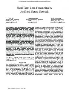
Fig. 2. An illustration of the novel distribution-level load forecasting method. In a subtree where Feeder 3 is the root node, nodes with shadowing are forecast by WNNs and the rest are forecast by LDFs.

Effects of switching operations on distribution-level load forecasting have been reported in [26] and [27]. A two-stage bad data identification method was developed in [27] to retrieve the historical trend of load and to improve the bus load forecasting by identifying and restoring inaccurate measurements and abnormal disturbance. A synergistic integration of Statistical Process Control (SPC) and Kalman filter was presented in [28] to detect faults of chillers and cooling coils by monitoring system parameters. The SPC was applied to evaluate variations of parameter predictions while Kalman filter was used to provide predictions and adaptive SPC control limits. The above detection methods captured abnormal changes effectively and could be adopted to detect switching operations. III. NEURAL NETWORKS AND LOAD DISTRIBUTION FACTORS Our new forecasting approach is presented in this section. Section III-A presents a WNN-based load forecasting method for a root node. Section III-B describes a criterion to classify child nodes as “regular” and “irregular” based on load pattern similarities. The LDF method to forecast load of a regular node is expressed in Section III-C. Section III-D introduces the WNN with appropriate inputs for irregular nodes. As illustrated in Fig. 2, load of the root node Feeder 3 in a given subtree is first forecast by the WNN. According to the results of node classification, the forecasts are distributed to regular nodes (transformers 1 and 3) by using LDF while the load of the irregular node transformer 2 is forecast by using WNN. Load forecasts of customers 1–3 are then obtained in the same manner by treating transformer 2 as a new parent node. A. Load Forecasting for a Root Node Previously, we have developed a WNN-based load forecasting method for large areas [15], [29]. The structure consists of similar day-based input selection, multi-level wavelet decomposition, and individual neural networks for different frequency components. The forecasting model for a root load follows this structure with modifications on input selection and the learning algorithm as depicted in Fig. 3. Inputs to WNNs include similar day load, previous day load, forecast weather, and day of week index while outputs are forecast loads of the next day at all time instances. The wavelet technique is used to decompose the data into three orthogonal components at different frequencies: Low-low (LL), Low-high (LH) and High (H). This process helps capture load features of individual

This article has been accepted for inclusion in a future issue of this journal. Content is final as presented, with the exception of pagination. 4

Fig. 3. The WNN-based load forecaster for a root node.

IEEE TRANSACTIONS ON POWER SYSTEMS

(1) where subscripts and , respectively, denote a forecast day and a historical day in the historical set ; subscripts and , respectively, denote the day before the forecast day and the day before the historical day ; represents the weather factor under consideration, i.e., wind-chill temperature if tomorrow is a winter day, and humidex if tomorrow is a summer day; represents the load and is the number of time instances during one day. , which is the average value of the historical load, is used to scale the magnitude of load differences. The weight of the load difference term is determined by the following minimization process on all historical days: (2) denotes the selected similar day load with pawhere rameter of a historical day at time instance ; denotes the actual load of day at time instance ; and is the number of historical days. Profiles of a substation actual load, original and modified similar day loads, and previous day (Day-1) load are depicted in Fig. 5. The mean absolute percent error (MAPE) and correlation coefficient with respect to the actual load are used to evaluate these load input variables according to (3)

Fig. 4. Load versus wind-chill temperature, humidex, and wind speed.

and components. Results of individual NNs are then summed to form the final forecasts. 1) Input Selection: To effectively capture features of the distribution-level load and forecast the next day load, inputs are properly selected. Day of week index is an important input factor because different days of the week have different load curves. Beyond that, weather is the major driver for load. Following [15], predicted wind-chill temperature and humidex on the next day are selected as weather input variables in WNNs. As shown in Fig. 4, approximate piecewise linear relationships exist between substation load and selected weather factors. Other weather factors such as wind speed, which has a highly nonlinear pattern and a weak correlation with the load, are not selected. In the method we previously developed for system-level load forecasting [15], similar day load is selected based on weather similarity and day of week index. Distribution-level load, which could be dominated by a few large customers, may vary with similar weather conditions and the same day of week index. Therefore, only considering weather similarity may not be sufficient. Typically, if the day before a weather-similar day also has a similar load curve with the day before a forecast day, the selected similar day load would better represent the forecast day load. The criteria of similar day selection (4) in [15] are thus modified according to

(4) where denotes the actual load, represents the load input variable to be examined, is the number of historical samples, and are the sample means. The MAPE measures the closeness between the input load and the target load while the correlation coefficient measures the association between the input load and the target load. As summarized in Table I, modified similar day load has the lowest MAPE and the highest correlation coefficient compared with other two load input variables. This indicates that the modified similar day load could better represent the load of a forecast day compared with the other two load input variables. Meanwhile, to anchor the selected similar day load and provide an initial status of the next day load, previous day load is supplemented to the modified similar day load. Numerical testing of different combinations of weather and load input variables are provided in Section V to verify the above selection. 2) Wavelet Neural Network: Combination of wavelet transform and NNs has been successfully used in load forecasting [15], [30], [31]. Unlike Fourier transform, which represents the signal as a sum of sinusoids localized in frequency only, wavelet transform uses basis functions which contain both time and frequency information. It is thus appropriate to use wavelet

This article has been accepted for inclusion in a future issue of this journal. Content is final as presented, with the exception of pagination. SUN et al.: AN EFFICIENT APPROACH TO SHORT-TERM LOAD FORECASTING AT THE DISTRIBUTION LEVEL

Fig. 5. Load curves of actual load, previous day load, original similar day, and modified similar day load.

TABLE I COMPARISONS OF LOAD INPUT VARIABLES WITH TARGET OUTPUT LOAD

5

cause information loss in the frequency domain. The Db members tested are Db2-Db20 (even index only), in which the index number refers to the filter length. To choose a good decomposition level and filter window length, extensive experiments are conducted [29]. Two-level decomposition with Db4 is found to be the best among levels from zero to three and DB index members from 2–20. Determination of the above parameters as well as the parameters in NNs such as the number of hidden neurons is through training, validation, and test processes in a three-way data split [33]: 1) Divide the data into training, validation and test sets; 2) Select one parameter (e.g., number of hidden neurons) and set values of other parameters to nominal levels. 1) Initialize the selected parameter; 2) Train WNN using the training set; 3) Evaluate the model on the validation set by calculating the validation set error; 4) Tune the parameter and repeat steps 2.2 and 2.3; 5) Select the parameter value which results in the minimum validation set error; 3) Repeat step 2 to determine other parameters; 4) Select the best model and train it using data from the training and validation sets; 5) Assess the final model using the test set. B. Node Classification

Fig. 6. Multiple-level wavelet decomposition scheme .

transform to deal with signals with nonstationary characteristic through multi-resolution analysis. Wavelet transform can be implemented by a filter bank presenting decomposition and reconstruction stages as shown in Fig. 6. In the decomposition stage, approximation and detail coefficients of an input signal are produced by convolving with filters and then by down-sampling. An ‘approximation’ holds the general trend of the original signal, whereas a ‘detail’ depicts high frequency component of it. In the reconstruction stage, wavelet coefficients are padded zeros (up-sampling) to recover the data length and are then convolved with reconstruction filters . Filters , , , and have to satisfy perfect reconstruction and orthogonality [32]. The input load is thus broken into low and high frequency components. A multilevel decomposition process can be achieved by successively decomposing the approximations. In this paper, a two-level wavelet composition is adopted. Thus, load and weather data are decomposed into LL, LH and H frequency components as the scheme presented. When these decomposed components are fed into individual NNs trained by node-decoupled EKF, the same forecasting quality is assumed for each component. The three forecasts are therefore summed with equal weights to obtain the final forecast. Daubechies (Db) wavelets are selected in our method because they are a family of orthogonal wavelets, and will not

Load pattern of a child node generally follows the pattern of its parent node. As weekly load profiles of a substation and its six feeders shown in Fig. 7, most feeders have similar load patterns with that of the substation. Nevertheless, there also exist deviations on particular days (e.g., Day 3 and Day 4) when load patterns of some feeders are different from that of the substation. The load pattern similarities motivate forecasting child nodes by the proportion from the parent load forecast. However, for those child nodes whose loads significantly vary from the parent load, proportion is not suitable and individual models are needed. To identify which category that a child node belongs to and select a proper forecasting method, a dynamic node classification method is developed. Similarity between two time series is commonly identified by distance matrix [34]–[36]. In [34], similarity matching of two observed series was based on the distance of wavelet coefficients after decomposing the data series. In [35] and [36], simple Euclidean distance was used to investigate the pattern similarities. In our problem, considering the different magnitudes of child nodes, Euclidean distance between the normalized child load and parent load is calculated as a pattern similarity index. Furthermore, since loads having the same day of week index are likely to have similar patterns, the distance between a child node and its parent node on day is estimated as the averaged distance of past weeks having the same day index with the forecast day as expressed in

(5) and

This article has been accepted for inclusion in a future issue of this journal. Content is final as presented, with the exception of pagination. 6

IEEE TRANSACTIONS ON POWER SYSTEMS

The LDFs are updated on each forecast day and this dynamic feature helps capture changes of the proportions. Load forecasts of a regular child node are then obtained simply as (9) and are load forecasts of child node where and its parent node, respectively. D. Load Forecasting Method for Irregular Nodes

Fig. 7. Load profiles of (a) a substation and (b) six feeders during a week from March 5, 2012 (Monday) to March 11, 2012 (Sunday).

(6) where

is the number of child nodes, and are the normalized loads of child node and the parent node at time instance on day , respectively. Distances between all child nodes and the parent node are calculated using (5) and (6). Node classification is then determined for the forecast day according to: ,

(7)

is a distance threshold. On each forecast day, a child where node is defined as “regular” if is smaller than the threshold; otherwise, it is defined as “irregular”. The threshold is initialized as the average of historical distances, and then tuned through training and validation data sets. This distance-based classification method can be treated as a simplified form of -means clustering in which the normalized parent load is the cluster center. Compared with the standard -mean clustering with two clusters, our classification calculates the distance between child and parent nodes and indicates how much the child loads follow the parent load. Numerical results for the estimated distances, actual distances, and the threshold distance are shown in Section V to verify and evaluate the classification. C. Load Forecasting Method for Regular Nodes To forecast the load of a regular node on day , LDFs are estimated by the averaged LDFs of the past weeks having the same day of week index with the forecast day as in (8)

For irregular nodes, since their load patterns could be significantly different from that of the parent node, LDF is not suitable. To better capture the complicated load features and estimate the nonlinear relationships between affecting factors and the target load, WNN-based forecasting model is used. In spatial load forecasting, correlations with neighboring regions and information available outside the target area are used to improve the forecasting accuracy [5]. Using information available from a neighboring area to predict a target area has achieved improvements in load forecasting [37], wind power forecasting [38] and solar power forecasting [39]. As discussed above, in addition to the inputs considered for a root node, load from correlated sibling nodes would help WNNs capture the load features of irregular nodes. Since the number of correlated nodes could be large, and if all are considered, algorithm complexity will increase and forecasting accuracy may even degrade. Our idea is to select one key sibling node and use the previous day load of this selected node as additional inputs to WNNs. IV. DETECTING SWITCHING OPERATIONS This section deals with detecting switching operations and adjusting forecasting methods after an identified switching operation. Section IV-A presents an SPC-based method to detect switching operations. In Section IV-B, the methods for adjusting LDFs and WNNs are described. A. An SPC-Based Method for Detecting Switching Operations Statistical Process Control (SPC) is used to monitor the actual load and detect abnormal changes according to load forecast means and standard deviations. If there is no switching operation, the actual load generally falls into a normal range. When a switching operation happens, actual load may exceed the normal range, causing significant changes to be caught by SPC rules. This switching operation detection method adopts the SPC-based detection idea and the SPC control rule from [28], in which a synergistic integration of SPC and Kalman filter was presented to detect the faults of chillers and cooling towers. Load forecast errors are commonly assumed to be Gaussian distributed [40]. Under this assumption, actual load falls into the one-sigma range with approximate 68% probability and two-sigma range with 95% probability without switching operations. In [28], two-sigma range is used as the adaptive SPC control limit to guarantee 95% Gaussian coverage. Similarly, a switching operation in the distribution system is detected if back-to-back points fall outside of the two-sigma range and the points are either all above upper limits or all below lower limits. This is because a switching operation typically keeps the trend and lasts for a certain period. The number of points, , is

This article has been accepted for inclusion in a future issue of this journal. Content is final as presented, with the exception of pagination. SUN et al.: AN EFFICIENT APPROACH TO SHORT-TERM LOAD FORECASTING AT THE DISTRIBUTION LEVEL

7

V. NUMERICAL TESTING The above method has been implemented in MATLAB on an Intel Core 2.20 GHz personal computer. The forecasting performance is evaluated by using the standard mean absolute percentage error (MAPE): (11)

Fig. 8. Dynamic two-sigma range as SPC control limits for detecting switching operations.

If the denominator error (MAE) is used:

in (11) is close to zero, mean absolute

(12) set to be 3 so that a potential switching operation is detected at the 99.99% confidence level according to (10) in [28]. For nodes forecast by WNN, standard deviations of the forecasts can be directly obtained from the diagonal elements of the innovation covariance matrix in decoupled EKF [18]. For regular nodes forecast by LDFs, standard deviations are derived approximately from those of their parent nodes. Assume that the load forecasting error of a parent node is Gaussian with standard derivation on day at time instance . The load forecasting error of its regular child node is then approximately obtained as a Gaussian with standard derivation proportioned by LDF from (10) Distributions of forecasting errors from WNN and LDF are analyzed to verify the normal assumption by Quantile-Quantile plots of the errors and sigma coverage rates of the actual load as demonstrated in the numerical testing. B. Adjusting LDFs and WNNs After the actual load of a forecast day is available, the load is examined using the SPC control rule as discussed above. If no switching operation is detected and no earlier switching operation is identified, regular forecasting processes will be followed for the next day. If a switching operation is detected and the load is switched back to the normal range, i.e., the abnormality does not last long, regular forecasting processes will be followed. If a switching operation is detected and it lasts until the end of the current day as shown in Fig. 8, adjusting LDFs or WNNs is needed. For a regular node, after such a switching operation, we keep on using LDF but the calculation in (8) is based on the latest new data only without the requirement of using data with the same day index. When the length of the new data collected is more than weeks, original LDF is used. However, after a switching operation is identified, a regular node may not maintain the regular pattern. Thus, WNN is started at the background with the new data until it is shown that the new pattern is regular, or WNN is ready to forecast. For an irregular node, after switching operations, we keep on using WNN with weights updated by the new data. Since the irregular node may become regular, LDFs are started with the new data at the background until it is shown that the new pattern is irregular, or when LDFs begin to produce good predictions.

Two practical datasets are tested in Examples 1 and 2, respectively. For both examples, one-year load data in 30-minute interval and hourly weather data are collected. The test set is the last month data, the validation set is one month prior to the test month, and the rest data are used for WNN training. When the validation error (MAPE/MAE) increases for five iterations, the training is stopped, and the weights resulting in the minimum validation error are stored. Parameters need to be set in WNNs, node classification, and LDF calculation are determined based on training and validation processes as described in Section III-A-2. Since only actual weather data are available, in the training period, actual weather data are used as WNN inputs whereas in the validation and testing periods, actual weather data plus a Gaussian noise are used as weather predictions. The forecasting performance of using this predicted weather is expected to be close to that in the real applications. Example 1: This example demonstrates load forecasting for a substation and six feeders located in a large city in North Carolina, United States. Load and weather data collected are from August 01, 2011 to July 24, 2012. The training period is from August 2011 to May 2012, the validation period is June 2012, and the test period is July 01–24, 2012. Seven cases are presented below. Case 1 demonstrates the learning and generalization capability of WNN using one-year data for substation load forecasting. Case 2 shows the values of input selection of WNN for substation load forecasting. Case 3 examines the dynamic feeder classification. Case 4 shows load forecasting for regular feeders. Case 5 compares WNN and LDF for irregular feeders. Case 6 evaluates the normal assumption for load forecasting errors and demonstrates the significance of switching operation detection. In Case 7, the performance of our method is compared with two naïve benchmarks, two multiple linear regression models, and one NN model. Case 1: The training and validation processes of each frequency component for substation load are described in this case. The inputs selected for WNN include similar day load, previous day load, forecast day weather predictions (wind-chill temperature and humidex), and day of week index. The training and validation errors are evaluated by MAPE for LL frequency component and MAE for LH and H components. As shown in Fig. 9, for LL frequency component, both training and validation processes converge quickly after several iterations. For LH and H frequency components, because the components are volatile,

This article has been accepted for inclusion in a future issue of this journal. Content is final as presented, with the exception of pagination. 8

IEEE TRANSACTIONS ON POWER SYSTEMS

NUMBER

OF

TABLE II HIDDEN NEURONS AND MAPE (%) FOR SUBSTATION JULY, 2012 LOAD (CASE 2-1 IN EXAMPLE 1)

M1: With wind-chill temperature; M2: With humidex; M3: With wind speed; M4: With both wind-chill temperature and humidex; M5: With wind-chill temperature, humidex and wind speed. TABLE III MAPE (%) FOR SUBSTATION JULY, 2012 LOAD (CASE 2-2 IN EXAMPLE 1)

Fig. 9. Training and validation errors with the number of training iterations for each frequency component. (a) LL frequency component; (b) LH frequency component; (c) H frequency component.

convergences are not as smooth as for the low frequency component. The validation set stops the training at a specific number of iterations if further five iterations on training data degrade the network generalization ability on the validation set. The numbers of iterations to meet the minimum validation errors are 22, 10, and 7 for LL, LH and H frequency NNs, respectively. Case 2: This case demonstrates the benefits of input weather and load variable selection for WNN to forecast the substation load. In our method, the inputs selected for WNN to forecast the load of a root node include similar day load, previous day load, forecast day weather predictions (wind-chill temperature and humidex), and day of week index. 1) Weather input variables: WNNs using different combinations of weather input variables are compared. Other inputs include similar day load, previous day load, and day of week index. MAPEs presented in Table II show the values of selected wind-chill temperature and humidex. 2) Load input variables: WNNs using different combinations of load input variables are compared. Other inputs include weather predictions (wind-chill temperature and humidex), and day of week index. The MAPEs presented in Table III show the values of selected load inputs. 3) Actual weather verse predicted weather: WNN using the actual weather and predicted weather on forecast days are compared. Results in Table IV show that with adding a noise on the actual weather, the forecasting MAPE increases compared with using actual weather. This is reasonable because using actual weather without uncertainties could result in lower MAPE. However, the performance of using weather data with uncertainty is expected to be close to the performance in the real applications. Case 3: The node classification process is presented in this case. In Table V, the first row shows the actual averaged distances calculated during the validation period June 2012 while the rest are the estimated distances on the last two weeks of the

M1: With previous day load; M2: With original similar day load; M3: With modified similar day load; M4: With both previous day load and original similar day load; M5: With both previous day load and modified similar day load. TABLE IV MAPE (%) FOR SUBSTATION JULY, 2012 LOAD (CASE 2-3 IN EXAMPLE 1)

test period. The distance threshold is set as 0.50, which is determined based on the historical actual distances and training-validation process. It can be seen that Feeders 1, 2, 3 and 5 are identified as “regular” nodes for all test days and they are forecast by LDF. Feeder 4 is identified as an “irregular” node for most of the test days. Even though the estimated distances on some days (e.g., July 16 and 17 with ) show regularity of Feeder 4, since this regularity does not keep long, WNN is still used until a long-term regularity is identified. As for Feeder 6, it has only one day identified as an irregular node during all test days. In view of the fact that the averaged distance during validation period shows the regularity of this node, and the irregularity did not keep long, Feeder 6 is therefore treated as a regular node and forecast by LDF for all test days. Thus five of six feeders are forecast by LDFs, which indicates a low computational effort. Actual distances during the last two weeks of the test period are also calculated for verification as shown in Table VI. The actual distances are generally consistent with the estimated and this demonstrates the overall irregularity of Feeder 4 and the regularity of other feeders. Case 4: Load Forecasting for regular nodes Feeders 1, 2, 3, 5 and 6 by using LDF and individual WNN are compared. The results summarized in Table VII show that the LDF captures load features and provides competitive load forecasts for regular nodes compared with the results from WNNs. Case 5: Load forecasting performance for an irregular node is shown in this case. Irregular node Feeder 4 is forecast by WNN with considering correlations with the selected sibling node Feeder 3. Three other approaches are compared: using WNN without considering correlations with other nodes, using WNN

This article has been accepted for inclusion in a future issue of this journal. Content is final as presented, with the exception of pagination. SUN et al.: AN EFFICIENT APPROACH TO SHORT-TERM LOAD FORECASTING AT THE DISTRIBUTION LEVEL

TABLE V ESTIMATED DISTANCES OF THE NORMALIZED LOADS BETWEEN SIX FEEDERS AND SUBSTATION (CASE 3 IN EXAMPLE 1)

9

TABLE VIII MAPE (%) FOR FEEDER 4 JULY, 2012 LOAD (CASE 5 IN EXAMPLE 1)

M1: Using WNN with a correlated sibling load as additional inputs; M2: Using WNN without any load inputs outside this node; M3: Using WNN with the substation load as additional inputs; M4: Using LDF.

TABLE VI ACTUAL DISTANCES OF THE NORMALIZED LOADS BETWEEN SIX FEEDERS AND SUBSTATION (CASE 3 IN EXAMPLE 1)

Fig. 10. Quantile-Quantile plot of substation load forecasting errors versus the standard normal.

Fig. 11. Quantile-Quantile plots of forecasting errors versus the standard normal for a regular load Feeder 1 and an irregular load Feeder 4.

TABLE VII MAPE (%) FOR REGULAR FEEDERS JULY, 2012 LOAD (CASE 4 IN EXAMPLE 1)

with the substation load as additional inputs, and using LDF method. Forecasting MAPEs are summarized in Table VIII. For Feeder 4, our method (M1) produces the lowest MAPE 7.25 as compared with other two WNNs and LDF. Case 6: This case verifies the normal assumption of the forecasting errors and demonstrates the switching operation detection. As shown in Fig. 10, Quantile-Quantile plot of the substation load forecasting errors clearly shows heavier tails than the

Gaussian. The Quantile-Quantile plots of load forecast errors for a regular node Feeder 1 and an irregular load Feeder 4 are also depicted in Fig. 11. Both have heavier tails than Gaussian. However, if the top and bottom tails are removed, the remaining errors follow a normal distribution. The standard deviation (STD) of the prediction, one-sigma and two-sigma actual load coverage rates calculated for substation and feeders are shown in Table IX. The one-sigma coverage rates range from 69.18% to 81.07%, which are slightly larger than 68% under the Gaussian assumption. The two-sigma coverage rates of all feeders are lower than the value 95% under Gaussian distribution. This is mainly because of the abnormal consumption occurred on July 2 for Feeder 1 and on July 8 for almost all feeders. These changes are caught by the two-sigma rule as shown in Fig. 12 for Feeder 1. The two-sigma coverage rates of the actual load are thus lowered. Because the abnormal load was switched back to the normal ranges, no adjustments are made in this case. Case 7: This case compares our method with two naïve benchmarks, two multiple linear regression (MLR) models, and one back propagation NN (BPNN). The naïve benchmarks include using previous day load (Day-1) and the load of a week ago (Day-7) as forecasts for the next day load. The first MLR

This article has been accepted for inclusion in a future issue of this journal. Content is final as presented, with the exception of pagination. 10

IEEE TRANSACTIONS ON POWER SYSTEMS

TABLE IX MAPES (%), MAES (MW), STDS (MW), ONE-SIGMA COVERAGE RATES (%), AND TWO-SIGMA COVERAGE RATES (%) FOR SUBSTATION AND FEEDER LOADS (CASE 6 IN EXAMPLE 1)

TABLE X MAPE (%)

FOR SUBSTATION AND FEEDER JULY, LOADS (CASE 7 IN EXAMPLE 1)

2012

A: Using our method ; D-1: Using previous day load; D-7: Using the load of a week ago; MLR (1): Using MLR with selected similar day load; MLR (2): Using MLR without selected similar day load; BPNN: Using back propagation NN.

Fig. 12. The switching operations detected for Feeder 1 on July 2 and July 8.

model has the corresponding independent variables as input factor of WNN as expressed in (13): (13) •

denotes the load at time instance . denotes the modified similar-day load at time instance . denotes the load of previous day at the same time instance for 30-minute data. • and denote predicted wind chill temperature and humidex at time instance , respectively. • is the day index: 1 for Monday, 2 for TuesdayWednesday-Thursday, 3 for Friday, 4 for Saturday, and 5 for Sunday. • is the time instance index, ranging from 1 to 48 for 30-minute data. • is the coefficient of each independent variable. • is i.i.d Gaussian random variable with zero mean and finite variance. The second MLR model has the same formulation but does not contain the modified similar day load variable. A traditional BPNN (implemented by MATLAB Neural Network Toolbox) without wavelet decomposition is also considered for comparison. Input factors for BPNN are identical with those used in WNN. Forecasting MAPEs for the substation and six feeders are summarized in Table X. As can be seen, benchmarks using previous day load and the load of a week ago encounter high prediction errors. The MLR without considering the similar day load also results in high MAPEs. However, when modified similar day load is taken into account, the prediction power of MLR is enhanced significantly. The MAPEs obtained from a single

BPNN further outperforms MLRs because the nonlinear representation of input-output relationship in NN can better capture the load characteristics than the linear relationship used in MLR. Overall, our method achieves the lowest MAPEs for both substation and feeders because it captures the complicated load features through wavelet decomposition and dynamic pattern similarity analysis. Moreover, when compared with the forecasting MAPEs ranging from 2% to 20% for substation and feeder loads reported in the literature [24], [25], our results are competitive. The NNs are trained offline by the historical data. Averagely, the training can be conducted within 20 minutes for both WNN and BPNN. Training times for WNN and BPNN are similar because even though BP iteration is faster than the decoupled EKF, BP converges much slower and requires a larger number of iterations. Once the WNN model is well trained and validated, it can be used to predict the next day load given the new input data. The weights of WNNs are then updated online with the realized latest 24 hours' loads. Example 2: This example demonstrates load forecasting for four feeders and selected customers in a city in Washington, United States. Load and weather data from December 01, 2011 to November 30, 2012 are collected. The training period is from December 2011 to September 2012, the validation period is October 2012, and the test period is November 2012. In addition, data of more than 1000 smart meters within this substation are available for four days from April 1, 2012 (a Sunday) to April 4, 2012. Two cases are presented below. Case 1 predicts substation and feeder loads. Case 2 extends the forecasting to the customer level. In both cases, inputs for WNNs include similar day load, previous day load, weather predictions on the forecast day (wind-chill temperature and humidex), and day of week index. Case 1: This case predicts substation and feeder loads and demonstrates the values of switching operation detection. Among four feeders, Feeders 1 and 2 are forecast by LDF while Feeders 3 and 4 are forecast by WNN. As shown in Fig. 13, a significant switching operation was detected on November 20, 2012 for Feeder 1. The load magnitude after switching operation decreased and Feeder 1 maintained the regular pattern for a certain period. Therefore, Feeder 1 is forecast by the original LDF for the first twenty test days. After November 20, Feeder

This article has been accepted for inclusion in a future issue of this journal. Content is final as presented, with the exception of pagination. SUN et al.: AN EFFICIENT APPROACH TO SHORT-TERM LOAD FORECASTING AT THE DISTRIBUTION LEVEL

11

are obtained. Simple and fast LDF method is applied to forecast the load of regular child nodes, whereas WNNs with correlated sibling node are used for irregular nodes. The SPC-based switching operation detection is also considered to improve the forecasting accuracy. Testing results demonstrate the high prediction accuracy of this method. The new approach represents an effective way to forecast distribution-level load and would be helpful in the future smart grid.

Fig. 13. Switching operations detected for Feeder 1 on November 20, 2012.

TABLE XI MAPE (%) FOR SUBSTATION AND FEEDER NOVEMBER, 2012 LOADS (CASE 1 IN EXAMPLE 2)

ACKNOWLEDGMENT The authors would like to thank Dr. David Sun and Mr. Brice Glenn at Alstom Grid as well as Mr. Anthony Williams and Mrs. Leslie Ponder at Duke Energy. The authors would also like to thank the editor and reviewers for their constructive comments and suggestions to improve the quality of this paper. REFERENCES

A: Using our method ; D-1: Using previous day load; D-7: Using the load of a week ago; MLR (1): Using MLR with selected similar day load; MLR (2): Using MLR without selected similar day load; BPNN: Using back propagation NN. TABLE XII MAPE (%) FOR SMART METER NOVEMBER, 2012 LOAD (CASE 2 IN EXAMPLE 2)

1 is forecast by the modified LDF, which is calculated based on the new data after the switching operation. Forecasting results of our method, two naïve benchmarks, two MLRs, and a simple BPNN are summarized in Table XI. It can be seen that our method provides the lowest MAPEs for the substation and all feeders. Case 2: Smart meter-based customer load is predicted in this case. Since the smart meter data are limited and no transformer data are available, predictions are generated by using LDFs. Hourly load of April 4, 2012 is forecast based on feeder load forecasts and LDFs calculated by smart meter readings of the previous two days (Sunday April 1 is ignored). Forecasting results of four selected customers are shown in Table XII. Because of the complicated customer behaviors and the limited data, the law of large number is not as effective as for the aggregated load. Thus, high MAPEs are obtained as expected. VI. CONCLUSION This paper presents a generic approach for short-term load forecasting at the distribution level within the hierarchical structure. With a root node forecast by WNNs and load pattern similarity-based child node classification, forecasts of all child nodes

[1] H. K. William, Distribution System Modeling and Analysis, 3rd ed. Boca Raton, FL, USA: CRC Press, 2011. [2] M. E. Baran, L. A. A. Freeman, F. Hanson, and V. Ayers, “Load estimation for load monitoring at distribution substations,” IEEE Trans. Power Syst., vol. 20, no. 1, pp. 164–170, Feb. 2005. [3] M. E. Baran and F. F. Wu, “Network reconfiguration in distribution system for loss reduction and load balancing,” IEEE Trans. Power Del., vol. 4, no. 2, pp. 1401–1407, Apr. 1989. [4] M. S. Tsai and F. Y. Hsu, “Application of grey correlation analysis in evolutionary programming for distribution system feeder reconfiguration,” IEEE Trans. Power Syst., vol. 25, no. 2, pp. 1126–1133, May 2010. [5] H. L. Willis, Spatial Electric Load Forecasting, 2nd ed. New York, NY, USA: Marcel Dekker, 2005. [6] Electric load forecasting [Online]. Available: http://www.quanta-technology.com/sites/default/files/doc-files/Load_Forecasting-12-0113.pdf [7] R. Sevlian and R. Rajagopal, “Value of aggregation in the smart grids,” in Proc. IEEE Int. Conf. Smart Grid Commun., Oct. 2013. [8] J. S. Taylor and N. Cristianini, Kernel Methods for Patter Analysis. Cambridge, U.K.: Cambridge Univ. Press, 2004. [9] D. Sun, K. Cheung, K. Chung, and T. Mckeag, “System Tools for Integrating Individual Load Forecasts Into a Composite Load Forecast to Present a Comprehensive Synchronized and Harmonized Load Forecast,” U.S. Patent 0035071, Feb. 10, 2011. [10] W. Guan, K. Chung, K. W. Cheung, X. Sun, L. D. Michel, S. Corbo, and P. B. Luh, “Advanced load forecast with hierarchical forecasting capability,” in Proc. IEEE Power and Energy Society General Meeting, Vancouver, BC, Canada, Jul. 2013. [11] I. Moghram and S. Rahman, “Analysis and evaluation of five shortterm load forecasting techniques,” IEEE Trans. Power Syst., vol. 4, no. 4, pp. 1484–1491, Nov. 1989. [12] Y. Bar-Shalom, X. R. Li, and T. Kirubarajan, Estimation With Applications to Tracking and Navigation: Theory Algorithms and Software. Hoboken, NJ, USA: Wiley, 2001. [13] S. Haykin, Neural Networks and Learning Machines, 3rd ed. Englewood Cliffs, NJ, USA: Prentice Hall, 2009. [14] A. Khotanzad, E. Zhou, and H. Elragal, “A neuro-fuzzy approach to short-term load forecasting in a price-sensitive environment,” IEEE Trans. Power Syst., vol. 17, no. 4, pp. 1273–1282, Nov. 2002. [15] Y. Chen, P. B. Luh, C. Guan, Y. G. Zhao, L. D. Michel, M. A. Coolbeth, P. B. Friedland, and S. J. Rourke, “Short-term load forecasting: Similar day-based wavelet neural networks,” IEEE Trans. Power Syst., vol. 25, no. 1, pp. 322–330, Feb. 2010. [16] S. Singhal and L. Wu, “Training feedforward networks with extended Kalman filter algorithm,” in Proc. Int. Conf. ASSP, 1989, pp. 1187–1190. [17] S. Haykin, Kalman Filtering and Neural Networks. Hoboken, NJ, USA: Wiley, 2001. [18] L. Zhang, P. B. Luh, and K. Kasiviswanathan, “Neural network-based market clearing price prediction and confidence interval estimation with an improved extended Kalman filter method,” IEEE Trans. Power Syst., vol. 120, no. 1, pp. 59–66, Feb. 2005.

This article has been accepted for inclusion in a future issue of this journal. Content is final as presented, with the exception of pagination. 12

IEEE TRANSACTIONS ON POWER SYSTEMS

[19] M. Espinoza, J. Suykens, R. Belmans, and B. D. Moor, “Electric load forecasting,” IEEE Control Syst. Mag., vol. 27, no. 5, pp. 43–57, Oct. 2007. [20] S. Fan and Y. Wu, “Multiregion load forecasting for system with large geographical,” IEEE Trans. Ind. Applicat., vol. 45, no. 4, pp. 1452–1459, Jul./Aug. 2009. [21] S. Fan, K. Methaprayoon, and W. J. Lee, “Short-term multi-region load forecasting based on weather and load diversity analysis,” in Proc. 39th North Amer. Power Symp., 2007, pp. 562–567. [22] N. Amjady, “Short-term bus load forecasting of power systems by a new hybrid method,” IEEE Trans. Power Syst., vol. 22, no. 1, pp. 333–341, Feb. 2007. [23] M. Espinoza, C. Joye, R. Belmans, and B. De Moor, “Short-term load forecasting, profile identification, customer segmentation: A methodology based on periodic time series,” IEEE Trans. Power Syst., vol. 20, no. 3, pp. 1622–1630, Aug. 2005. [24] Y. Goude, R. Nedellec, and N. Kong, “Local short and middle term electricity load forecasting with semi-parametric additive models,” IEEE Trans. Smart Grid, vol. 5, no. 1, pp. 440–446, Jan. 2014. [25] K. N. Filho, A. D. P. Lotufo, and C. R. Minussi, “Short-Term multimodal load forecasting using a general regression neural network,” IEEE Trans. Power Del., vol. 26, no. 4, pp. 2862–2869, Oct. 2011. [26] J. Yasuoka, J. L. P. Brittes, H. P. Schmidt, and J. A. Jardini, “Artificial neural network-based distribution substation and feeder load forecast,” in Proc. 16th Int. Conf. Elect. Distribution, 2001. [27] X. Chen, C. Kang, X. Tong, Q. Xia, and J. Yang, “Improving the accuracy of bus load forecasting by a two-stage bad data identification method,” IEEE Trans. Power Syst., vol. 29, no. 4, pp. 1634–1641, Jul. 2014. [28] B. Sun, P. B. Luh, Q. S. Jia, Z. O'Neill, and F. Song, “Building energy doctors: An SPC and Kalman filter-based method for system-level fault detection in HVAC systems,” IEEE Trans. Automat. Sci. Eng., vol. 11, no. 1, pp. 215–229, Jan. 2014. [29] C. Guan, P. B. Luh, L. D. Michel, Y. Wang, and P. B. Friedland, “Very short-term load forecasting: Wavelet neural networks with data prefiltering,” IEEE Trans. Power Syst., vol. 28, no. 1, pp. 30–41, Feb. 2013. [30] R. R. Agnaldo and P. A. Alexandre, “Feature extraction via multiresolution analysis for short-term load forecasting,” IEEE Trans. Power Syst., vol. 20, no. 1, pp. 189–198, Feb. 2005. [31] N. Amjady and F. Keynia, “Short-term load forecasting of power systems by combination of wavelet transform and neuro-evolutionary algorithm,” J. Energy, vol. 34, no. 1, pp. 46–57, Jan. 2009. [32] G. Strang and T. Nguyen, Wavelets and Filter Banks, 2nd ed. Wellesley, MA, USA: Wellesley-Cambridge Press, 1997. [33] R. Gutierrez-Osuna, Lecture 13: Validation [Online]. Available: http:/ /research.cs.tamu.edu/prism/lectures/iss/iss_l13.pdf [34] A. Antoniadis, E. Paparoditis, and T. Sapatinas, “A functional waveletkernel approach for time series prediction,” J. Royal Statist. Soc. B, vol. 68, pp. 837–857, Nov. 2006. [35] E. Keogh, K. Chakrabarti, M. Pazzani, and S. Mehrotra, “Dimensionality reduction for fast similarity search in large time series databases,” Knowl. Inf. Syst., 2001. [36] P. Esling and C. Agon, Time-Series Data Mining, ACM Computing Surveys, Dec. 2012. [37] C. Gu, D. Yang, P. Jirutitijaroen, W. M. Walsh, and T. Reindl, “Spatial load forecasting with communication failure using time-forward kriging,” IEEE Trans. Power Syst., vol. 29, no. 6, pp. 2875–2882, Nov. 2014. [38] D. A. Bechrakis and P. D. Sparis, “Correlation of wind speed between neighboring measuring stations,” IEEE Trans. Energy Convers., vol. 19, no. 2, pp. 400–406, Jun. 2004. [39] S. Pelland, G. Galanis, and G. Kallos, “Solar and photovoltaic forecasting through post-processing of the global environmental multiscale numerical weather prediction model,” Progr. Photovoltaics: Res. Applicat., vol. 21, no. 3, pp. 284–296, May 2013. [40] B. M. Hodge, D. Lew, and M. Milligan, “Short-Term load forecasting error distributions and implications for renewable integration studies,” in Proc. 2013 IEEE Green Technologies Conf., Denver, CO, USA, Apr. .

Xiaorong Sun (S'12) received her Bachelor degree in Electrical Engineering from Hohai University, Nanjing, China, in 2010. She is currently a Ph.D. student in the Electrical & Computer Engineering Department in the University of Connecticut, Storrs, CT, USA.

Her research interests include electricity load and price forecasting, transmission and distribution systems, and power system optimization.

Peter B. Luh (S'77–M'80–SM'91–F'95) received his BS from National Taiwan University, MS from MIT, and Ph.D. from Harvard University. He has been with the Department of Electrical and Computer Engineering at the University of Connecticut, Storrs, CT, USA since 1980, and is the SNET Professor of Communications & Information Technologies. He is also a member of the Chair Professors Group at the Center for Intelligent and Networked Systems (CFINS) in the Department of Automation at Tsinghua University, Beijing, China; and a Chair Professor in the Department of Electrical Engineering, National Taiwan University, Taipei, Taiwan. His research interests include smart, green and safe buildings; smart grid, electricity markets, and effective renewable integration to the grid; and intelligent manufacturing systems. Prof. Luh was the founding Editor-in-Chief of the IEEE TRANSACTIONS ON AUTOMATION SCIENCE AND ENGINEERING, and an EiC of the IEEE TRANSACTIONS ON ROBOTICS AND AUTOMATION. He is the recipient of the 2013 Pioneer Award of the IEEE Robotics and Automation Society for his pioneering contributions to the development of near-optimal and efficient planning, scheduling, and coordination methodologies for manufacturing and power systems.

Kwok W. Cheung (S'87–M'91–SM'98–F'14) received his Ph.D. in Electrical Engineering from Rensselaer Polytechnic Institute, Troy, NY, USA in 1991. He joined ALSTOM Grid Inc. (formerly ESCA) in 1991 and is currently Director, R&D of Network Management Solutions focusing on innovation and technology. His current interests include electricity market design and implementation, smart grid, renewable energy integration, energy forecasting, power system stability and micro grid. Dr. Cheung has been a registered Professional Engineer of the State of Washington since 1994.

Wei Guan (M'12) received her doctoral degree in mathematics from the University of Oklahoma. She is a power system engineer at Alstom Grid Inc. Previously she worked as research scientist at the School of Electrical and Computer Engineering at the University of Oklahoma. Her current research interest is in the electricity market management system and related smart grid product solutions.

Laurent D. Michel received the M.S. and Ph.D. degrees in computer science from Brown University, Providence, RI, USA in 1996 and 1999, respectively. He is an Associate Professor of computer science and engineering at the University of Connecticut, Storrs, CT, USA. His interests span combinatorial optimization with a particular emphasis on constraint programming, load forecasting, and voting technology. He has co-authored two monographs and more than 80 papers.

S. S. (Mani) Venkata (M'68–SM'77–F'89–LF'08) is currently a Principal Scientist at Alstom Grid. He has taught for more than 38 years at five different universities. He is an author or co-author of more than 350 technical publications and/or presentations.

Melanie T. Miller received the B.S. degree in computer engineering from UNCC and an MBA from Wingate University. She has 15 years of experience with Duke Energy where she has had the opportunity to have positions in several organizations. Currently, she is the Director of Technology Performance and Optimization. In her previous role, she was responsible for understanding the impacts distributed energy resources will have on the distribution and transmission grid and evaluating new technologies associated with distributed resources, real time operations, distribution automation, and data analytics. She was also the project manager for the deployment of energy storage, PV, PEVs, communication nodes, PMUs, and line sensors in the Envision Energy Project in Charlotte, NC, USA.