660
IEEE TRANSACTIONS ON SYSTEMS, MAN, AND CYBERNETICS-PART B: CYBERNETICS, VOL. 26, NO. 4, AUGUST 1996
An Extended Procedure of Constructing Neural Networks for Supervised Dichotomy
11. THE LEARNING RULE Suppose we have a set D of training examples. Each example in D is represented by the following data structure:
Shie-Jue Lee and Mu-Tune Jone
Abstruct- Cios and Liu [l] proposed a neural network generation procedure for supervised two-class discretization based on a continuous ID3 algorithm. The method constructs neural networks consisting of neurons with linear activation functions. We extend the procedure to allow decision boundaries to he any arbitrary function. The advantage of the extension is revealed by the decrease in size of the generated neural networks.
1. INTRODUCTION
When building a neural network for classification, we are confronted with the determination of the number of hidden layers and the number of nodes in each hidden layer. Kung and Hwang [2] used the algebraic projection analysis to specify the size of hidden layers. Nadal [ 3 ] ,Bichsel and Seitz [4], and Cios and Liu [ l ] used entropy to determine the number of hidden layers and the number of nodes in each hidden layer. These methods are all based on neurons whose activation functions are first-order polynomials [5]. Although the obtained neural network can solve a nonlinearly separable problem, its size could be huge [6]. Neurons with high-order activation functions are more powerful than neurons with linear activation functions [ 7 ] , [8]. Therefore, a neural network built on the neurons of the former kind may have smaller numbers of hidden layers and nodes in each hidden layer than a neural network built on the neurons of the latter kind. Take the famous XOR problem as an example. It's well known that at least one hidden node is needed if we use neurons with linear decision boundaries, as shown in Fig. 1. However, by applying an output node with an activation function of second-order polynomial, no hidden layer is needed as shown in Fig. 2. We extend the neural network generation procedure proposed by Cios and Liu [l]. Instead of assuming linear activation functions, we allow decision boundaries to be any arbitrary function. As in [ I ] , minimal numbers of hidden layers and nodes in each hidden layer are determined by minimizing the information entropy function associated with the partition induced by activation functions. A leaming process combining the delta rule and a Cauchy-based simulated annealing method is developed to obtain the coefficients of optimal decision boundaries. An experiment is done on spiral data and shows that a neural network built on neurons with activation functions of second-order polynomial not only has a smaller number of nodes in each layer but also has a smaller number of hidden layers than that built on neurons with linear activation functions. The experiment also shows that the partition formed by second-order decision boundaries is smoother than that formed by first-order decision boundaries.
struct example { F an array of real numbers; e: a binary number:
1 Semantically, F' = ( ~ ' 1 . ' . U , ) denotes the n attribute values associated with an example; and c denotes the class that the example belongs to, I for positive class and 0 for negative class. For convenience, we will use e . 3 to represent all attribute values of the example e , e . ( ' , to represent the ,jth attribute value of e , and c.c to represent the category of e. For a subset S of D , we define the class entropy of S to be: ~
where S, and S, are subsets of S containing examples of positive and negative classes, respectively, and S = S p U Srz.Note that denotes the number of elements in X . Suppose D is partitioned into R subsets, d l , . . . , dn, denoted by {c&}:=~, by a number of hypersurfaces. The information entropy [9]-[ 121 associated with {drj!Ll is
1x1
R Itl
E({d,}fz=,j = 1'=
I
I I(&).
ID1
Suppose we want to refine { d, jFzl by adding one more hypersurface Hit?. 2) where ti? represents the coefficients (u1, . . ., tunL and I represents the variables SI, ..., .rn. Let the resulting regions after In order to express the role of H(tZ, 2) addition be {d,.}:ll. explicitly, we write {d, = { d r } ~ z l / H ( t Z.?). , The information entropy associated with {dr}:L1 is
}Fll
R'
= r=l
-Id,I (I & ) . /Dl
The entropy gain we obtain is
, )in a more desirable way. Let each We can express { d F } f = l / H ( G I set d,. in { d r } F Z l be divided by H ( G , 2) into two subsets: d d and d:, such that d: = { e E d T I H ( G ,e.5)
> 0},
(1: = { e E d,lH(iu'. e.a)
5 0).
Since d: and d> are disjoint, the following relations hold: Manuscript received April 24, 1994; revised March 31, 1995. This work was supported by National Science Council under Grant NSC-83-0408-E110-004. The authors are with the Department of Electrical Engineering, National Sun Yat-Sen University, Kaohsiung 80424, Taiwan, R.O.C. (emai1:
[email protected]). Publisher Item Identifier S 1083-4419(96)03938-6.
d, = d z U d, = d,>p U d:n
+ I&.
Id71 = ldrpl d: = d, - (d:,
U d,>)
ldr'l =Id.I - ld?,l - I d 2 = d r p - dr', I d & = ldrpl
d5n
=a,,
-
-
IePl
clzn
ICnI = Idrn I - len I. And (1) becomes
E
[
H
]
Given a set D of training examples, if 1) is partitioned into R subsets, such that all the examples in any region belong to the same class, then E ( { d y ) ~ = l )= 0. However, we want to find a minimal number of hypersurfaces for such a partition. Our ,algorithm is as follows. Starting from the original set D of training examples, we find a hypersurface H ( 6 , 2) to divide Ll into two regions d l and i l 2 such that E [ D / H ( w ' ,Z ) ] is minimized. If the entropy of i.he two regions is 0, then we are done. Otherwise we find another hypersurface to divide the set D further, and so on. The process can be described in the following algorithm. procedure Search-0ptimal:Hypersurfaces let d = D ;
U = {I; while E ( d ) # 0 do find a hypersurface H ( 6 . Z ) which minimizer; E[d/H(71?,Z ) ] ; li = U U {H(w'. .':I}; let d be the set of data regions resulting from the addition of H(w". ,F); endwhile end Search-Optimal_Hypersuirfaces. How do we find the hypersurface H ( 6 . 2) which minimizes E [ d / H ( w ' ,Z)]in the above algorithm? An exhaustive search is obviously impossible. A delta rule which searches for global minima 1131 is used.
IEEE TRANSACTIONS ON SYSTEMS, MAN, AND CYBERNETICS-PART
662
B. CYBERNETICS, VOL 26, NO. 4, AUGUST 1996
I
I
X Fig. 2.
Y
Solving the XOR problem using neurons with nonlinear activation functions.
For each coefficient t u j IT: in H(tC. .?), we initialize it to some ) . we modify it each time value. Let the initial value be ~ ~ ( 0Then by adding an amount which is proportional to the gradient of the information entropy. That is
+
exp [-H(d. ?)]}-I. Let the output function of a neuron, {I be denoted by O [ H ( d . The values of /cl$] and ldz7zl can be calculated by
?)I.
*
(1
-
O [ H ( G .e.')]}
* d H (dww' ,Je.Z)
J
~
IEEE TRANSACTIONS ON SYSTEMS, MAN, AND CYBERNETICS-PART
B: CYBERNETICS, VOL. 26, NO. 4, AUGUST 1996
663
TABL,E I DIFFERENT TYPESOF HYPERSURFACES -
COMPARISON OF NEURAL NETWORKS WITH
first-order
cross terms
cross terms
Fig. 3. Spiral data set. which optimally refines the regions, {dr}:zi=l, can be obtained by the following algorithm: procedure DeltaRule initialize all wJ E cu'; while E({dr}F=l/H[w', Z ) ] is not minimized d o U J = ~ wJ A w J , for all tul E ?U'; endwhile end DeltaRule.
+
Unfortunately, the delta rule approach usually has a problem of being trapped to local minima. As in [l], a fast simulated annealing strategy, called the Cauchy machine [14], is used to escape from local minima.
Fig. 4. Data regions generated by first-oriier hypersurfaces Ti
* (1 - O [ H ( 6 .e..')]} *
111. POLYNOMIALS AS HYPERSURFACES
(e.luk)i~ k=l
Suppose H ( G . 2) is a polynomial of order m and dimension n:
A. Hyperplanes Parallel to Axes where Il. . . . , I,, are nonnegative integers and W I , I , is the coefficient for the term z : (Le., z f l zp . . . z?). Then we have
n,"=,
Traditional continuous ID3 [12] applies a hyperplane of the following form
H(cu', Z)
z=
z3
+8
to the ,jth attribute and uses exhaustive search to find an optimal 0. This can be done by using our delta rule: R
A8 = - 7
{O[H(G,
e.ir)]
* (1 - O [ H ( Z ,2 . F ) ] )
r=l e t d ,
B. General First-Order Hypersu$bces If we set m = 1, then H ( G . rr') becomes k=l
R
A w l , ... I , = -7
{ O [ H ( , Z :e..')] r=l ?Ed,
/
n
\
664
IEEE TRANSACTIONS ON SYSTEMS, MAN AND CYBERNETICS-PART
B CYBERNETICS, VOL 26, NO 4, AUGUST 1996
which can be rewritten to
The delta rule for A u J .1 5 j
5 n , can be simplified to
R
AB =the same as (2) which is the Cios and Liu’s continuous ID3 algorithm [ l ]
C. Second-Order Hypersurfaces
If we take m = 2. then H ( G . 2) becomes Fig. 5. Data regions generated by second-order hypersurfaces without cross terms. a neural network to classify D is described below [l].
which can be rewritten to
procedure BuiIdNeuralNetwork
specify the order of hypersurfaces, m ; set Din? to be the number of attributes of input examples; i + 0; do
it-i+l;
Then the delta rule can be simplified to
* (1 - O[H(72. f.?)]}
‘i
using the procedures Search-Optimalllypersufaces and DeltaRule to generate s hypersurfaces of dimension Dim; create s nodes correspondingly and these nodes form the ith hidden layer; each node in the ith hidden layer connects to the input nodes and the nodes of all previous hidden layers; Dim + Dim +s; until s = 1 end BuildNeuralNetwork.
(e.v3)2
* (1 - O[H(w’.e..‘)]} * ( e . ? , ) * ( e . 1 . k ) V. COMPARISON A”.,
= the same as (3)
A0 = t h e same as (2).
We present some experimental results and give a comparison for neural network architectures with different types of hypersurfaces. The data set D we use is shown in Fig. 3 which contains the following two sets of spiral data: spiral-1:
IV. BUILDINGNEURALNETWORKS When a hypersurface H(7B. 5) is found using the approach described in Section 11, a neuron is created corresponding to this hypersurface. As we mentioned, a sequence of hypersurfaces divide a data set into a desired number of regions. The neurons each of which corresponds to one hypersurface of the sequence form a hidden layer. However, we want a single node for the output, with the output value being 1 for positive examples and 0 for negative examples. Therefore, we have to generate as many hidden layers, with each neuron connecting to the original inputs and the outputs of all previous hidden layers, until we have a layer with only one neuron. Given a set D of training examples, the process of building
spiral-0: where
c c
21
= p cos ( e )
YI = p sin (0) x2 y2
= - p cos ( e ) = - p sin ( 8 )
p = cu8, 0=
0.125,
0 . 2 5 ~5 0 5 S K . Each element in the set spiral-1 is a positive example (denoted by “+” in the figure), i.e., belonging to class 1. Each element in the set spiral-0 is a negative example (denoted by “-” in the figure), i.e.,
IEEE TRANSACTIONS ON SYSTEMS, MAN, AND CYBERNETICS-PART
B: CYBERNETICS, VOL. 26, NO. 4, AUGUST 1996
665
arbitrary function. As in [1], minimall numbers of hidden layers and nodes in each hidden layer are determined by minimizing the information entropy function associated with the partition induced by hypersurfaces. A learning process, combining the delta rule and a Cauchy-based simulated annealing strategy, foir obtaining the coefficients of optimal hypersurfaces is also described. We have also indicated that Traditional continuous ID3 and (30s and Liu’s continuous ID3 are special cases of our method. An experiment is done on spiral data to show that a neural network built with second-order hypersurfaces not only has a smaller number of nodes is each layer but also has a smaller number of hidden layers than that built with first-order hypersurfaces. The experiment also shows that the partition formed by. second-order hypersurfaces is smoother than that formed by first-order hypersurfaces
ACKNOWLEDGMENT Comments from anonymous referees are appreciated.
REFERENCES Fig. 6. Data regions generated by second-order hypersurfaces with cross terms. belonging to class 0. There are 125 points in each class, making 250 examples totally in D . We want to compare the performance of neural networks with the following three types of hypersurfaces: I) First-order. 2) Second-order without cross terms. 3) Second-order with cross terms. Hypersurfaces of second-order with cross terms have more terms than hypersurfaces of second-order without cross terms, but they can slant and thus may result in a smaller number of neurons. Hypersurfaces of second-order without cross terms are interesting since they have C,” fewer coefficients than hypersurfaces of secondorder with cross terms and only twice more coefficients than firstorder hypersurfaces. Comparison of these three types for the set D is shown in Table I. Clearly, the neural network architecture with first-order hypersurfaces is most complicated. It has two levels of hidden layers having 35 and 8 nodes, respectively, 411 connections among neurons, and 455 coefficients in the hypersurface functions. The architecture with second-order hypersurfaces having no cross terms has the smallest number of coefficients, while the architecture with second-order hypersurfaces having cross terms has the smallest numbers of nodes and connections. Data regions dividing the training examples space obtained from different architectures are shown in Figs. 4-6, respectively. Shaded regions are for negative examples (class 0) and nonshaded regions are for positive examples (class 1). The hypersurfaces of each architecture 100% correctly separate the data set D . However, regions generated by second-order hypersurfaces are smoother than those generated by first-order hypersurfaces. It should be noted that our algorithm is applicable to any set of data with continuous or discrete values. At the present, the structure of hypersurfaces has to be provided by the user. It would be nice if the structure of hypersurfaces, such as the order, with or without cross terms, etc., could be determined automatically. VI. CONCLUSION We have extended the neural network generation procedure proposed by Cios and Liu [l], to allow decision boundaries to be any
[ 11
[2] [3] [4] [5] [6] [7] [8]
[9] [ 101
[I11 1121 [13] [ 141
K. J. Cios and N. Liu, “A machine learning method for generation of a neural network architecture: A continuous ID3 algorithm,” IEEE Trans. Neural Networks, vol. 3, pp. 280-290, 1992. S. Y. Kung and J. N. Hwang, “An algebraic prcijection analysis for optimal hidden units size andl learning rates in back-propagation learning,” in Proc. IEEE Int. Con$ Neural Networks, 1988, pp. 363-370. J. P. Nadal, “New algorithms for feedforward networks,” in Neural Networks and SPIN Classes, Theumann and Koberle, E.ds. New York: World Scientific, 1989, pp. 80-88. M. Bichsel and P. Seitz, “Minimum class entropy: A maximum information approach to layered networks,” Neural Networks, vol. 2, pp. 133-141, 1989. F. Rosenblatt, “The perceptron: A probabilistic model for information storage and organization in the brain,” Psychol. Rev., vol. 65, pp. 42-99, 1958. K. Lang and M. J. Witbrock, “Learning to tell two spirals apart,” in Proc. Connectionist Models Summer School, 1988, pp. 52-59. C. C. Chiang and H. C. Fu, “On the capability of a new perceptron for two-class classification problerns,” J. Inform. Sci. Eng., vol. 8, pp. 567-585, 1992. S. Y. Kung, Digital Neural Networks. Englewood Cliffs, NJ: PrenticeHall, 1993. J. R. Quinlan, “Induction of decision irees,” Machine JLearning, vol. 1, no. I , pp. 81-106, 1986. I. Kononenko and I. Bratko, “Information-based evaluation criterion for classifier’s performance,” Machine Leurning, vol. 5 , pp. 67-79, 1989. G. L. Bilbro and D. E. V. Bout, “Maximum entropy and learning theory,” Neurul Comp., vol. 4, pp. 839-853, 1992. U. M. Fayyad and K. B. Irani, “O’n the handling of continuous-valued attributes in decision tree generation,” Machine Leanzing, vol. 8, pp. 87-102, 1992. L. Wessels, E. Barnard, and E. ven FLooyen, “The physical correlates of local minima,” in Proc. Int. Neurul Networks Cor$, Paris, France, July 1990, pp. 985-992. H. Szu and R. Hartley, “Fast simulated annealing,” P,kys. Lett. A , vol. 122, pp. 157-162, 1987.