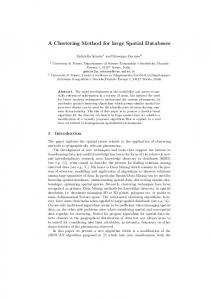
An Extensible Index for Spatial Databases

An Extensible Index for Spatial Databases Walid G. Aref and Ihab F. Ilyas Department of Computer Sciences, Purdue University West Lafayette IN 47907-1398 aref,ilyas @cs.purdue.edu


Abstract Emerging database applications require the use of new indexing structures beyond B-trees and R-trees. Examples are the k-D tree, the trie, the quadtree, and their variants. They are often proposed as supporting structures in data mining, GIS, and CAD/CAM applications. A common feature of all these indexes is that they recursively divide the space into partitions. A new extensible index structure, termed SP-GiST, is presented that supports this class of data structures, mainly the class of space partitioning unbalanced trees. Simple method implementations are provided that demonstrate how SP-GiST can behave as a kD tree, a trie, a quadtree, or any of their variants. Issues related to clustering tree nodes into pages as well as concurrency control for SP-GiST are addressed. A dynamic minimum-height clustering technique is applied to minimize disk accesses and to make using such trees in database systems possible and efficient. A prototype implementation of SP-GiST is presented as well as performance studies of the various SP-GiST’s tuning parameters.

1. Introduction Emerging database applications require the use of new indexing structures beyond B+-trees. The new applications may need different index structures to suit the big variety of data being supported e.g., video, image, and multidimensional data. Example applications are cartography, CAD, GIS, telemedicine, and multimedia applications. For example, the quadtree [17, 28] is used in the Sloan Digital Sky Survey to build indexes for different views of the sky (a multi-terabyte database archive) [44], the linear quadtree [20] is used in the recently released Oracle spatial product [9], the trie data structure is used in [1] to index handwritten databases. The reader is referred to [9, 13, 15, 16, 19, 23, 37, 39, 42] for additional database applications that use different spatial and non-traditional tree structures.

Having a single framework to cover a wide range of these tree structures is very attractive from the point of view of database system implementation. Because of the need for non-traditional indexes, tree structures, e.g., quadtrees [17, 28], k-D trees [5], tries [10, 18], and Patricia tries [29] are now highly needed as index structures [19] to support emerging database applications. Designing a database indexing technique that has this flexibility of supporting various tree structure indexes is hindered by two main problems. The first problem is the storage/structure characteristics of spatial trees. Most of the unbalanced spatial tree structures are not optimized for I/O, which is a crucial issue for database systems. Quadtrees, tries, and k-D trees can be so skinny and long. Unless the problem of appropriately clustering the tree nodes into pages is addressed properly, this would lead to many I/O accesses before getting the required query answer. Compare this to the B+-tree, that in most cases has a height of 2-3 levels, and to the R-tree [24] and its variants, the R*-tree [4] and the R+-tree [43] that play an important role as spatial database indexes [6, 11, 38]. The second problem is the implementation effort of building indexes. Hard wiring the implementation of a full fledged index structure with the appropriate concurrency and recovery mechanisms into the database engine is a non-trivial process. Repeating this process for each spatial tree that can be more appealing for a certain application requires major changes in the DBMS core code. After all, one may still need a new structure that will cause, rewriting/augmenting significant portions of the DBMS engine to add the new tree index. The Generalized Search Tree (GiST) [25], was introduced in order to provide single implementation for B-tree-like indexes, e.g., the B+-tree [29], the R-tree [24], and the RD-tree [26]. Although practically useful, the class of unbalanced spatial indexes, e.g., the quadtree, the trie, and the k-D tree, is not supported by GiST because of the structure characteristics mentioned. One important common feature of the quadtree, the trie, and the k-D tree family of indexes is that at each level of the tree, the underlying space gets partitioned into disjoint partitions. For example, in the case of a two-dimensional

quadtree, at each level of decomposition, the space covered by a node is decomposed into four disjoint blocks. Similarly, in the case of the trie (assuming that we store a dictionary of words), the space covered by a node in the trie gets decomposed into 26 disjoint regions (each region corresponds to one letter of the alphabet). The k-D tree exhibits similar behavior. We use the term space-partitioning trees to represent the class of hierarchical data structures that decomposes a certain space into disjoint partitions. The number of partitions and the way the space is decomposed differ from one tree to the other. In this paper we study the common features among the members of the spatial space partitioning trees aiming at developing a framework that is capable of representing the different tree structures and overcoming the difficulties that prevent such useful trees from being used in database engines. The DBMS will then be able to provide a large number of index structures with simple method plug-ins. As demonstrated in the paper, for the framework of space partitioning trees, we furnish in the DBMS (only once) the common functionalities such as the insertion, deletion, and updating algorithms, concurrency control and recovery techniques and I/O access optimization. For example, in a multimedia or a data mining application, we may then freely choose the best way to index each feature depending on the application semantics. By writing the right extensions to the extensible single implementation, a quadtree, a trie, a k-D tree, or other spatial structures can be made available without messing with the DBMS internal code. The rest of the paper is organized as follows. Section 2 presents the class of space-partitioning trees. In Section 3, the SP-GiST framework is presented. Section 3 also includes a description of SP-GiST external user interface, and illustrates the realization of various tree structures using it. This includes a realization of the k-D tree and the Patricia trie. Section 4 gives the implementation of the internal methods of SP-GiST. Concurrency control and recovery for SP-GiST are discussed in Section 5. Node clustering in SPGiST is presented in Section 6. Implementation and experimental results for the various tuning parameters of SP-GiST are given in Section 7. Section 8 contains some concluding remarks.

2. The Class of Space Partitioning Trees The term space-partitioning tree refers to the class of hierarchical data structures that recursively decomposes a certain space into disjoint partitions. It is important to point out the difference between data-driven and spacedriven decompositions of space. If the principle of decomposing the space is dependent on the input data, it is called data-driven decomposition, while if it is dependent solely on the space, it is called space-driven decomposi-

tion. Examples of the first category are the k-D tree [5] and the point quadtree [28]. Examples of the second category are the trie index [10, 18], the fixed grid [35], the universal B-tree [3], the region quadtree [17], and other quadtree variants (e.g., the MX-CIF quadtree [27], the bintree, the PM quadtree [41], the PR quadtree [36] and the PMR quadtree [34]). There are common underlying features among these spatial data structures. The term quadtrie was introduced in [39] to reflect the structure similarity between the trie and the quadtree. Similarly, the k-D tree and the MX quadtree have many structural similarities, e.g., both structures recursively partition the space into a number of disjoint partitions. On the other hand, the two trees differ in the number of partitions to divide the space and also in the decomposition principle. The decomposition is data-driven in the case of the k-D tree, while it is space-driven in the case of the MX quadtree. The structural and behavioral similarities among many spatial trees create the class of space-partitioning trees. In contrast, the differences among these trees enable their use in a variety of emerging applications. The nature of spatial data that the application is dealing with, as well as the types of queries that need to be supported, aid in deciding which space-partitioning tree to use. Space-partitioning trees can be differentiated on the following basis: Structural differences
 : Type of data they represent.
 : Decomposition fan-out (number of partitions).
 : Resolution (variable or not).
 : Structure constraints (allowing single child).
 : The use of buckets (allowing more than one data item to reside in a tree node) Behavioral differences   : The decomposition principle (data or space driven partitioning). The structural differences or design options can be viewed as Shape Parameters for the realized tree. For example, in the realization of the PR quadtree or more
 precisely  the PR-quadtrie, the represented data is “point” ( ). The decomposition depends on the space not on the data inserted  (compare to the k-D tree) ( ). Each time a partitioning
  of the space quadrant into four equal quadrants ( and
 ) takes place to divide the quadrant that has two points so that each point is attached with one quadrant. The decomposition resolution is “variable” in the sense that the partitioning
stops  whenever one data point resides in the quadrant ( ). Figure 1 shows an example PR quadtree. At the leaf level, nodes can be “white” (i.e.,
contains no data   ) or “black” (i.e., contains one data point ( ) ).

3. SP-GiST Framework Interface

Figure 1. An example PR quadtree. Using the same analogy, we can analyze the structure and behavior of
the  trie. The data represented in a trie is of type “word” (   ). The decomposition of the trie is spacedependent (
 ), as we always decompose the space into 26 partitions ( ); one partition for each letter of the alphabet.
In one variant of the trie, the resolution is “not vari  able” ( ) as we need to decompose the space until we consume all the letters of the inserted word (refer to Figure 2a for illustration). This is in contrast to stopping the decomposition only when a space partition uniquely identifies the inserted word (see Figure 2b). The same analysis S

S

P

P

T

A

D

E

E

SPACE

R

STAR

3.1 Interface Parameters A

A

C

SP-GiST is a general index framework that covers a wide range of tree indexes representing the large class of spacepartitioning search trees represented in Section 2. The structural characteristics of space-partitioning trees that distinguish them from other tree classes are: (1) Spacepartitioning trees decompose the space recursively. Each time, a fixed number of disjoint partitions is produced. (2) Space-partitioning trees are unbalanced trees (3) Spacepartitioning trees suffer from limited fan-out, e.g., the quadtree has only a fan-out of four. So, space-partitioning trees can be skinny and long. (4) Two different types of nodes exist in a space-partitioning tree, namely, index nodes (internal nodes) and data nodes (leaf nodes). The framework reflects these facts by having two main parts; the internal tree methods that reflect the similarities among all members of the class of space-partitioning tree, and the external interface that enables us to identify the features specific to a particular tree reflecting the differences listed in Section 2. By specifying user access methods as in GiST [25], SPGiST has some interface parameters and methods that allow it to represent the class of space-partitioning trees and reflect the structural and behavioral differences among them.

SPACE

The following interface parameters are the way a user can realize a particular space-partitioning tree. SPADE

STAR

NodePredicate: This parameter gives the predicate to be used in the index
nodes  of the tree (addresses the structural difference ). For example, a quadrant in a quadtree or a letter in a trie are predicates that are associated with an index node.

SPADE (a)

(b)

Figure 2. Two variants of the trie data structure : (a) resolution is not variable (b) resolution is variable. can be applied to realize other quadtree and trie variants, the k-D tree, and the bin-tree. In the following sections, we will introduce a general framework, termed SP-GiST, where we can use it to implement a big collection of space-partitioning trees. SP-GiST has one core implementation as well as user plug-ins that reflect the required structural and behavioral characteristics. The existence of such a framework will facilitate the adaption of this class of space-partitioning trees into database engines.

Key Type: This parameter gives the type of the data in the leaf level of the tree. For example, “Point” will be the key type in an MX quadtree while “Word” will be the key type of a trie. The data type Point and the data type Word have to be pre-defined by the user. NumberOfSpacePartitions: This parameter gives the number of
disjoint partitions produced at each decom position ( ). It also represents the number of items in index nodes. For example, quadtrees will have four space partitions, a trie of the English alphabet will have 26 space partitions, the k-D tree will have only two space partitions at each decomposition. Resolution and ShrinkPolicy: Resolution is the maximum number of space decompositions and is set depending on the space and the granularity required. For space-partitioning trees, recursive decomposition can

lead to long sparse structures. Parameter ShrinkPolicy is useful in limiting the number of times the space is recursively decomposed in response to data insertion. ShrinkPolicy can be one of three different policies (refer to Figure 3 for an illustration of the use of ShrinkPolicy in the context of the trie): S

S

p

t

a

a

p

Star

a

d

c

e

e

Space

r

S

Space

Space

Star

pa

Spade

Spade

Star

ShrinkPolicy is the way the 
 framework
 uses to map and . As shown, the structural differences many variants of spatial tree can be realized according to these structural differences. BucketSize : This parameter gives the maximum number of data items a data node can hold. It also represents the Split Threshold for data nodes. For example, quadtrees have the notion of a bucket size that determines when to split a node (e.g.,
as in  the PMR quadtree [34]). The use of buckets ( ) is an attractive design options for many database applications where we are concerned about storing multiple data items per bucket for storage performance efficiency.

3.2. External Methods (Behavior)

Spade (a)

only child of the index node ”m” is the index node ”p”, both nodes are merged together to reduce path length.

(b)

(c)

Figure 3. The effect of the parameter ShrinkPolicy on the trie : (a) Never Shrink, (b) Leaf Shrink, and (c) Tree Shrink.

– Never Shrink: Data is inserted in the node that corresponds to the maximum resolution of the space. This may result in multiple recursive decompositions of the space. – Leaf Shrink: Data is inserted at the first available leaf node. Decomposition will not depend on the maximum possible resolution. In this strategy, no index node will have one leaf node as we decompose only when there is no room for the newly inserted data item.

The external methods are the second part of the SP-GiST interface that allows the user to specify the behavior of each tree.   The main purpose is to map the behavioral difference in Section 2. Note the similarity between the names of the first two methods and the ones introduced in the GiST framework [25] although they are different in their functionalities. Let E : (p, ptr) be an entry in an SP-GiST node, where p is a node predicate or a leaf data key and ptr is a pointer. When p is a node predicate, ptr points to the child node corresponding to its predicate. When p is a leaf data key, ptr points to the data record associated with this key.

– Tree Shrink: The internal nodes are merged together to eliminate all single child internal nodes. This strategy is adapted from structures like the Patricia trie that aim at reducing the height of the tree as much as possible.

Consistent(Entry E, Query Predicate q, level): A
Boolean function that is false when (E.p q) is guaranteed unsatisfiable, and is true otherwise. This method will be used by the tree search method as a navigation guide through the tree. Argument level is used in order to determine consistency depending on the current decomposition level. For example, in a quadtree, a query of a data point (x,y) is consistent only with the entry that points to the quadrant containing this point.

For example, in the case of ShrinkPolicy =“Never Shrink”, when storing the word “implementation” in the trie, the word will be stored in a leaf after a 14nodes path, one level per input character. On the other hand, in the case of ShrinkPolicy =“ Leaf Shrink”, the input word may be stored in a leaf after the three-node path “i”, “m”, “p”, and “lementation”, since based on the current words in the trie, splitting up to the letter “p” makes a unique leaf entry for the word “implementation”. Finally, in the case of ShrinkPolicy = “Tree Shrink”, the input word may be stored in a leaf after a three-node path “i”, “mp”, l, “ementation”. Since the

PickSplit(P, level, splitnodes, splitpredicates): Returns Boolean, where P is a set of BucketSize+1 entries that cannot fit in a node. PickSplit defines a way of splitting the entries into a number of partitions equal to NumberOfSpacePartitions and returns a Boolean value indicating whether further partitioning should take place or not. The parameter level is used in the splitting criterion because splitting will depend on the current decomposition level of the tree. For example, in a trie of English words, at level i, splitting will  be according to the i character of each word in the over-full node. PickSplit will return the entries of the

Chicago

split nodes in the output parameter splitnodes, which is an array of buckets, where each bucket contains the elements that should be inserted in the corresponding child node. The predicates of the children are also returned in splitpredicates.

Toronto Denver

Mobile

Buffalo Toronto Denver Buffalo Chicago Atlanta

Atlanta

Cluster(): This method defines how tree nodes are clustered into disk pages. The method is explained in more detail in Section 6.

Mobile

Figure 4. An example k-D Tree. The interface methods realize the behavioral design options listed in 2. Methods Consistent and PickSplit determine if the tree follows the space-driven or the data-driven partitioning. For example, in a k-D tree, which is a datadriven space partitioning tree, method Consistent compares the coordinates of the query point (the point to be inserted or searched for) against the coordinates of the point attached to the index node. The values of these coordinates are determined based on data that is inserted earlier into the k-D tree. On the other hand, method Consistent for a space-driven space partitioning tree, e.g., the trie, will only depend on the letters of the newly inserted word. The comparison is performed against the letter associated with the index node entry, which is space-dependent, and is independent of the previously inserted data. We can also show that method PickSplit completes the specification of the behavioral design option by specifying the way to distribute nodes entries among the produced partitions. Examples of PickSplit for various tree structures are given in Section 3.3.

Parameters

Consistent(E,q,level)

PickSplit(P,level)

Table 1. Realization of the k-D Tree using SPGiST.

3.3. Realization of Space-Partitioning Trees

The realization of the k-D tree is given in Table 1. ShrinkPolicy is set to ”Leaf Shrink” because we put each input point at the first available place depending on the previously inserted points. Each node will hold only one point, (BucketSize = 1). We have only two space partitions for the “right” and “left” to a point (NoOfSpacePartitions = 2 ).

Using the SP-GiST interface, given in the previous sections, we demonstrate how to realize some commonly used space-partitioning indexes. More specifically, we present the realization of the k-D tree and the Patricia trie. The realization of many other space partitioning trees including the trie and some quadtree variants can be found in [2]. The k-D tree: k-D trees [5] are a special kind of search trees, useful for answering range queries about a set of points in the k-dimensional space. The k-D tree uses a datadriven decomposition of the space (see Section 2). The tree is constructed by partitioning the space into two halves with respect to one of the dimensions at each tree level. The algorithm for the two-dimensional case (i.e., ) with points in the plane is as follows: The algorithm selects any point and draws a line through it, parallel to the -axis. This line partitions the plane vertically into two halfplanes. Another point is selected and is used to horizontally partition the half-plane in which it lies. In general, a point that falls in a region created by a horizontal partition will divide this region vertically, and vice versa. This division process induces a binary tree structure, (e.g.,see Figure 4).





ShrinkPolicy = Leaf Shrink BucketSize = 1 NoOfSpacePartitions = 2 Node Predicate = ”left”, ”right”, or blank. Key Type = Point IF (level is odd AND q.x satisfies E.p.x) OR (level is even AND q.y satisfies E.p.y) RETURN TRUE ELSE RETURN FALSE Put the old point in a child node with predicate ”blank” Put the new point in a child node with predicate ”left” or ”right”, RETURN FALSE






The Patricia Trie: A trie [10, 18] is a tree in which the branching at any level is determined by only a portion of the key. The trie contains two types of nodes; index and data nodes. In the trie of Figure 5, each index node contains 27 link fields. In the Figure, index nodes are represented by rectangles, while data nodes are represented by ovals. All characters in the key values are assumed to be one of the 26 letters of the alphabet. A blank is used to terminate a key value. At level 1, all key values are partitioned into 27 disjoint classes depending on their first character. Thus, LINK(T,i) points to a subtrie containing all key values be ginning with the letter (T is the root of the trie). On the   level the branching is determined by the character. When a subtrie contains only one key value, it is replaced by a node of type data. This node contains the key value, together with other relevant information such as the address of the record with this key value, etc. The Patricia trie [33, 29]





is a special trie structure. It has the property that all nodes which have only one arc are merged with their parent nodes. To avoid false matches each node in the Patricia trie must have either the counter for the number of eliminated nodes or a pointer to the eliminated symbols. For example, Figure 5 shows a trie and a particia trie with a bucket size of 2. Inserting the words, ”abate”,”abacus”, and ”abort” will cause node splitting in both trees in a different way.

root blank a b ......

0

ab blank a b ....o .........

a blank a b ...... abate, abacus

2

Consistent(E,q,level)

PickSplit(P,level)

Depth

1

Parameters

abort

b blank a b ....o .........

abate, abacus

ShrinkPolicy = Tree Shrink BucketSize = B NoOfSpacePartitions = 26 Node Predicate = letter or Blank Key Type = String IF (q[level] == E.letter) OR (E.letter == BLANK AND level length(q)) RETURN TRUE ELSE RETURN FALSE Find a Common prefix among words P Update level = level+length of the common prefix Let P predicate = the common prefix Partition data strings in P according to the character values at position “level” IF any data string has length level, insert data string in Partition “blank” IF any of the partitions is still over full RETURN TRUE ELSE RETURN FALSE




abort

Ordinary Trie

Patricia Trie

Figure 5. The Trie and the Patricia Trie. In the Patricia trie, unlike the k-D tree, data nodes can hold many data items, say ”B” items. This is because it is a space-driven space-partitioning tree. The number of space partitions is equal to the size of the alphabet set. When Nodepredicate is “BLANK”, this leaf node will hold all words of length equal to tree depth. ShrinkPolicy is set to “Tree Shrink”. When splitting a node, we search for the common prefix of all words, the common prefix is returned as the predicate of the parent node, while splitting is performed based on the next letter after that prefix. The realization of the Patricia trie using SP-GiST is given in Table 2.

4. SP-GiST Internal Methods The methods for insertion, deletion, and search in SPGiST are internal operations that are implemented inside the SP-GiST index engine. These methods are used in conjunction with the external methods to realize specific spacepartitioning trees. The user of SP-GiST provides only the external methods, while the internal methods are hard coded into the SP-GiST index engine. The internal methods are general for the class of space-partitioning trees, and their behavior is tuned by making use of the user-defined external methods and parameters. The internal methods are designed to accommodate for the space-partitioning, recursive decomposition, bucket sizes, insertion resolution, and node clustering (refer to the structural and behavioral characteristics of spacepartitioning trees, given in Section 2). Recall that unlike the GiST structure, SP-GiST has to

Table 2. Realization of the Patricia Trie using SP-GiST.

support two distinct types of nodes; index and data nodes. Index nodes (non-leaf nodes) hold the various space partitions at each level. Each entry in an index node is a root of a subtree that holds all the entries that lie in this partition. The space partitions are disjoint. Besides having a slot for each space partition, the index node contains an extra blank slot to point to data nodes attached to the partition represented by this node. On the other hand, data nodes (leaf nodes) hold the key data and other pointer information to physical data records. We can think of data nodes as Buckets of data entries. Thus, a splitting strategy determined by PickSplit will be applied to split over-full data nodes. The insert algorithm, given in Table 3, depends on the following interface parameters and external methods: (1) Parameter ShrinkPolicy specifies how deep we should proceed with the space decomposition. (2) Method Consistent specifies which branch to follow. (3) Method PickSplit to split over-full nodes. The return value of PickSplit tells us when we should stop the splitting process. Method Insert begins by checking Parameter ShrinkPolicy. If ShrinkPolicy is set to “Never Shrink”, method Insert performs a successive creation of index nodes to the maximum space resolution. If the parameter is set to “Leaf Shrink” or “Tree Shrink”, the insertion algorithm searches for the first leaf node with a predicate that is Consistent with the key to be inserted. In the case of “Tree Shrink”, some eliminated index nodes may be needed while locating the leaf. Hence, an internal split is performed to “expand” the eliminated index nodes. If the leaf node is over-full, then method PickSplit will be invoked continuously to distribute the entries among

ALGORITHM INSERT (TreeNode root, Key, level) CurrentNode =root /* Initially root is null */ (1)IF ShrinkPolicy is “Never Shrink” THEN LOOP WHILE level SpaceResolution AND level Key length IF node is NULL THEN E = Create a new node of type INDEX. FOR i=1 TO NumberOfSpacePartitions LOOP IF (Consistent(E[i],key,level)) THEN index=i CurrentNode = E[index].ptr. /* the child pointed by entry E[index]*/ level = level +1 (2)IF CurrentNode is INDEX node /* pick a child to go */ FOR i=1 TO NumberOfSpacePartitions LOOP IF (Consistent(E[i], key, level)) THEN index=i IF None Of them is consistent AND ShrinkPolicy is “Tree Shrink” THEN Compare the key with the CurrentNode predicate. IF there is a common prefix THEN Change CurrentNode predicate to the common prefix Create a new INDEX node. Let CurrentNode be the new index node. Repeat the search for a consistent entry. CurrentNode=CurrentNode[index].ptr INSERT (CurrentNode, key, level+1) /* recursive */ /* node is of type DATA and may need to be split*/ (3)IF CurrentNode is full THEN LOOP WHILE PickSplit(node,level) n=Create new node of type INDEX Create Children for the split entries Parent(n) = Parent(CurrentNode) Adjust branches of ’n’ to point to the new children. level = level +1 ELSE insert the key in CurrentNode /* not a full node */ (4)Cluster() /* to recluster the tree nodes in pages */ 



Table 3. SP-GiST insertion algorithm.

non over-full children or until it reaches the maximum resolution of the underlying space. Notice that method Insert invokes method cluster to dynamically re-cluster the nodes properly after insertion. Clustering is further explained in Section 6. The Search method in SP-GiST is exactly similar to that of the GiST scheme, and hence is not shown here for brevity (see [25]). Method Search uses method Consistent as the main navigation guide. Starting from the root, the algorithm will check the search item against all branches using the method Consistent till reaching leaf nodes. The algorithm for method Delete in SP-GiST uses logical deletion. Deleted items are marked deleted and are not physically removed from the tree. This will save the effort of reorganizing trees at each deletion specially, for datadriven space-partitioning trees. A rebuild is used from time to time as a clean procedure.

5. Concurrency and Recovery in SP-GiST Concurrency and recovery in GiST have been addressed in [8, 31]. In [31] the authors provide general algorithms for concurrency control in tree-based access methods as well as a recovery protocol and a mechanism for ensuring repeatable read isolation [21]. They suggest the use of Node Sequence Number (NSN) for concurrency control, first introduced in [30]. For SP-GiST, a split (only at the leaf level) transforms a data node into an index node. Data is then distributed among new leaf nodes rooted at that split node. This fact simplifies the concurrency control mechanism significantly. As an example, consider the case when a search for a key is interleaved with an insertion that causes the splitting of the target node. By the time the search reaches the target node, it can not falsely conclude the non-existence of the searched key (as in a B-Tree scenario), because the new node is an index node. In that case, no right links need to be maintained between leaves (refer to the B-link algorithm [32]). The search will need to continue deeper in the tree not on the siblings level. Thus, no special sequence number (as in GiST) is needed for the concurrent operation to know that the node in question has been split. The operation will directly continue working with the child nodes. Phantom protection in GiST has also been addressed in two different techniques. Predicate locking [14] is used in [31] while Chakrabarti and Mehrotra in [8] propose a dynamic granular locking approach (GL/GiST) to phantom protection. We adopt the granular locking technique since it is more preferable and less expensive than predicate locking. The fact that a “Containment Hierarchy” exists in space-partitioning trees, represented by SP-GiST, will make the algorithm introduced in [7, 8] highly applicable and much simpler. Hence, in SP-GiST, because the node predicates form a containment hierarchy, we simply use the node predicates for granular locks. The main difference in SP-GiST is that a page may contain multiple SP-GiST nodes. A clustering algorithm will hold the mapping between nodes and pages. In this context, we assume that the node size is smaller than or equal to the page size. Hence the problem transforms to locking on a finer granularity. Treating nodes clustered in pages as records, granular locks [22] are used. The recovery technique used in [31] is directly applicable to SP-GiST.

6. Node Clustering in SP-GiST Node clustering means choosing the group of nodes that will reside together in the same disk page. Considering physical storage of the tree nodes, a direct and simple implementation of a node is to assign a disk page for each

node. However, for very sparse nodes, this simple assignment will not be efficient for database use [12]. We provide to the user a default node clustering method that is shown to perform well in the dynamic case [12]. However, we allow the user to override the default clustering method and provide a different node clustering policy that is more suitable for the type and nature of the operations to be performed on the constructed index. This will enhance the query response time of SP-GiST. We propose the interface method Cluster for this purpose. Introducing new nodes in the tree structure will internally invoke the dynamic clustering algorithm defined in Cluster to reconstruct the tree disk page structure and reflect the change. However, for unexperienced users or for typical database applications, SP-GiST has a default node clustering algorithm that achieves minimum height and hence minimum I/O access. The dynamic clustering algorithm in [12] is a good clustering algorithm and we use it as our default in SP-GiST. The pseudo code and a brief outline of the clustering algorithm is given in [2]. The user can choose other clustering algorithms that reflect the application semantics specially for non-traditional data types like in multimedia databases or video databases. Some possibilities are: (1) Fill-Factor Clustering: Tries to keep each page half-full for space utilization efficiency. (2) Deep Clustering: Chooses the longest linked subtree from the collection of page nodes to be stored together in the same page. This will enhance performance for depthfirst traversal of trees. (3) Breadth Clustering: Chooses the maximum number of siblings of the same parent to be stored together in the same page.

tree. Setting ShrinkPolicy to “Leaf Shrink” will realize a common variant of the trie where data can be put in the first available node. On the other hand, if ShrinkPolicy is set to “Tree Shrink”, it will realize the Patricia implementation of the trie where no single-arc nodes are allowed. Figure 6 gives the effect of this parameter on the trie data structure for various settings of BucketSize for a dataset of 10000 records with “string” keys. As expected, for the trie and the Patricia trie, the path length and the number of pages improve as the bucket size increases since less splitting takes place. On the other hand, the bucket size does not have an effect on the original trie. In this case, splitting will take place not because of the bucket size limit but to decompose the space to the maximum resolution. In the case of the original trie, each record will fall in a single node regardless of the setting of the bucket size. For the quadtree, the same argument holds. Experimental results for point datasets of 10000 points are given in Figure 7. In this case, setting ShrinkPolicy to “Never Shrink” will have the effect of realizing the MX quadtree while setting it to “Leaf Shrink” will realize the PR quadtree where data can be put in the first available node. Experiments with setting ShrinkPolicy to “Tree Shrink” show the realization of another variant of quadtree, where all white nodes are eliminated [40], making it more attractive for databases and solving the problem of long degenerate quadtrees when the workload is highly skewed.

8. Conclusion

7. Implementation and Experimental Results We implemented SP-GiST using C++ on SunOS 5.6 (Sparc). As a proof of concept, using SP-GiST, we implemented the extensions for some data structures namely, the MX quadtree, the PR quadtree, the trie, and the Patricia trie. The implementation has proven the feasibility of representing space-partitioning trees using the interface proposed by SP-GiST and the settings in the tables in Section 3.3. We performed experiments on various settings of the tunable interface parameters; BucketSize and ShrinkPolicy. In our implementation we adopt the minimal Height clustering technique in [12]. Results show that applying this clustering technique reduces the path length in terms of pages significantly. As explained in Section 3.1, the interface parameter ShrinkPolicy can take one of three values; “Never Shrink”, “Leaf Shrink“, or “Tree Shrink”. For the trie, setting ShrinkPolicy to “Never Shrink” will have the effect of realizing the original trie, where splitting is performed to the maximum resolution of the space, leading to a long sparse

SP-GiST is a generalized space-partitioning tree implementation of a wide range of tree data structures that are not I/O-optimized for databases. This makes it possible to have single tree index implementation to cover various types of trees that suit different applications. Emerging database applications will require this availability of various index structures due to the heterogeneous collection of data types they deal with. SP-GiST is an interesting choice for multimedia databases, spatial databases, GIS, and other modern database systems. We have shown how to augment SP-GiST with parameters and methods that will enable the coverage of this class of space-partitioning trees. Clustering methods were also addressed to realize the use of these structures in practice, in non-traditional database applications. Concurrency and recovery for SP-GiST are addressed to enable the realization of SP-GiST in commercial database systems. Experiments proved the concept of SP-GiST and provided some insight on the effect of the tunable interface parameters on the tree structure and performance.

6.0 6000.0 Original Trie Trie Patricia Trie

4.0

Number of Pages (pages)

Number of Pages (pages)

5.0

3.0

2.0

Original Trie Trie Patricia Trie 4000.0

2000.0

1.0

0.0 0.0

10.0

20.0 Bucket Size

30.0

40.0

(a)

0.0 0.0

10.0

20.0 Bucket Size

30.0

40.0

(b)

Figure 6. Effect of BucketSize on maximum path length for different settings of ShrinkPolicy for the trie.

References [1] W. G. Aref, D. Barbar´a, and P. Vallabhaneni. The handwritten trie: Indexing electronic ink. In Proceedings of the 1995 ACM SIGMOD, San Jose, California, May 1995. [2] W. G. Aref and I. F. Ilyas. A framework for supporting the class of space-partitioning trees. Technical Report 01002, Department of Computer Sciences, Purdue University, March 2001. [3] R. Bayer. The universal B-tree for multidimensional indexing: General concepts. Lecture Notes in Computer Science, 1274, 1997. [4] N. Beckmann, H. P. Kriegel, R. Schneider, and B. Seeger. The R* -tree: an efficient robust access method for points and rectangles. SIGMOD Record, 19(2), 1990. [5] J. L. Bentley. Multidimensional binary search trees used for associative searching. Communications of the ACM, 19:509–517, 1975. [6] T. Brinkhoff, H.-P. Kriegel, and B. Seeger. Parallel processing of spatial joins using R-trees. In ICDE’1996, New Orleans, Louisiana, February 1996. [7] K. Chakrabarti and S. Mehrotra. Dynamic granular locking approach to phantom protection in R-trees. In ICDE’1998, Orlando, Florida, USA, pages 446–454, February 1998. [8] K. Chakrabarti and S. Mehrotra. Efficient concurrency control in multidimensional access methods. In SIGMOD 1999, Proceedings ACM SIGMOD, Philadephia, Pennsylvania, USA, pages 25–36, June 1999. [9] O. Corporation. Oracle spatial (data sheet). http://www.oracle.com/database/documents/spatialds.pdf, March 1999. [10] R. de la Briandais. File searching using variable length keys. In Proceedings of the Western Joint Computer Conference, pages 295–298, 1959.

[11] D. J. DeWitt, N. Kabra, J. Luo, J. M. Patel, and J.-B. Yu. Client-Server Paradise. In VLDB’1994, pages 558–569, Santiago, Chile, 1994. [12] A. A. Diwan, S. Rane, S. Seshadri, and S. Sudarshan. Clustering techniques for minimizing external path length. In VLDB’96, Mumbai (Bombay), India, pages 342–353, September 1996. [13] C. Esperanca and H. Samet. Spatial database programming using sand. Proceedings of the Seventh International Symposium on Spatial Data Handling, May 1996. [14] K. P. Eswaran, J. N. Gray, R. A. Lorie, and I. L. Traiger. The notions of concurrency and predicate locks in a data base system. Communications of the ACM, 19(11), 1976. [15] C. Faloutsos and V. Gaede. Analysis of n-dimensional quadtrees using the Hausdorff fractal dimension. In VLDB’1996, pages 40–50, 3–6 Sept. 1996. [16] C. Faloutsos, H. V. Jagadish, and Y. Manolopoulos. Analysis of the n-dimensional quadtree decomposition for arbitrary hyperectangles. TKDE, 9(3):373–383, 1997. [17] R. A. Finkel and J. L. Bentley. Quad trees: a data structure for retrieval on composite key. Acta Informatica, 4(1):1–9, 1974. [18] E. Fredkin. Trie memory. Commun. ACM, 3:490–500, 1960. [19] V. Gaede and O. Gunther. Multidimensional access methods. In ACM Computer Surveys, 30,2, pages 170–231, June 1998. [20] I. Gargantini. An effective way to represent quadtrees. Communications ACM, 1982, 25(12):905–910, 1982. [21] J. N. Gray. Notes on data base operating systems. In Springer Verlag (Heidelberg, FRG and NewYork NY, USA) LNCS, ’Operating Systems, an Advanced Course’, Bayer,Graham, Seegmuller(eds), volume 60. 1978. [22] J. N. Gray and A. Reuter. Transaction Processing: concepts and techniques. Data Management Systems. Morgan Kaufmann Publishers, Inc., San Mateo (CA), USA, 1993.

8.0 7.5 7.0

Number of Pages (pages)

6.5 Max Path length(pages)

MX−Quad PR−Quad Patricia Quad

4000.0 MX−Quad PR−Quad Patricia Quad

6.0 5.5 5.0 4.5 4.0 3.5

3000.0

2000.0

1000.0

3.0 2.5 2.0 0.0

10.0

20.0 Bucket Size (a)

30.0

40.0

0.0 0.0

10.0

20.0 Bucket Size (b)

30.0

40.0

Figure 7. Effect of BucketSize on maximum path length for different settings of ShrinkPolicy for the quadtree.

[23] R. H. G¨uting. An introduction to spatial database systems. VLDB Journal, 3(4):357–399, 1994. [24] A. Guttman. R-trees: a dynamic index structure for spatial searching. ACM SIGMOD, pages 47–57, June 1984. [25] J. M. Hellerstein, J. F. Naughton, and A. Pfeffer. Generalized search trees for database system. In proceedings of VLDB, 1995. [26] J. M. Hellerstein and A. Pfeffer. The RD-tree: An index structure for sets. Technical report, University of Wisconsin Computer Science, 1994. [27] G. Kedem. The quad-CIF tree: A data structure for hierarchical on-line algorithms. In ACM IEEE Nineteenth Design Automation Conference Proceedings, pages 352–357, Los Alamitos, Ca., USA, June 1982. [28] A. Klinger. Pattern and search statistics. In S. RUSTAGI Ed., Optimizing Methods in Statistics, pages 303–337, 1971. [29] D. E. Knuth. The Art of Computer Programming, Vol. 3. Addison-Wesley, Reading, 1973. [30] M. Kornacker and D. Banks. High-concurrency locking in R-trees. In VLDB’95, Zurich, Switzerland, Sept. 1995. [31] M. Kornacker, C. Mohan, and J. M. Hellerstein. Concurrency and recovery in generalized search trees. ACM SIGMOD, pages 62–72, May 1998. [32] P. L. Lehman and S. B. Yao. Efficient locking for concurrent operations on B-Trees. ACM Transactions on Database Systems, 6(4):650–570, Dec. 1981. [33] D. R. Morrison. PATRICIA - practical algorithm to retrieve coded in alphanumeric. J. Assoc. Comput. Mach., 15(4):514–534, 1968. [34] R. C. Nelson and H. Samet. A consistent hierarchical representation for vector data. In Computer Graphics (SIGGRAPH ’86 Proceedings), volume 20(4), Aug. 1986.

[35] J. Nievergelt, H. Hinterberger, and K. Sevcik. The grid file: an adaptable symmetric multi-key file structure. ACM Transactions on Database Systems, 9(1):38–71, 1984. [36] J. A. Orenstein. Multidimensional tries used for associative searching. Information Processing Letters, 14(4):150–157, June 1982. [37] J. A. Orenstein and F. Manola. PROBE spatial data modeling and query processing in an image database application. IEEE Transactions on Software Engineering, 14(5):611– 629, May 1988. [38] D. Papadias, N. Mamoulis, and V. Delis. Algorithms for querying by spatial structure. In VLDB’98, New York City, New York, USA, pages 546–557, August 1998. [39] H. Samet. Applications of Spatial Data Structures. AddisonWesley, 1990. [40] H. Samet. The Design and Analysis of Spatial Data Structure. Addison-Wesley, 1990. [41] H. Samet and R. E. Webber. Storing a collection of polygons using quadtrees. ACM Transactions on Graphics, Volume 4, Issue 3, 1985. [42] B. Seeger and H.-P. Kriegel. The Buddy-tree: An efficient and robust access method for spatial data base systems. In VLDB’1990, August 1990,Queensland, Australia, Proceedings, 1990. [43] T. Sellis, N. Roussopoulos, and C. Faloutsos. The R+ tree: A dynamic index for multi-dimensional objects. In VLDB’1987, Brighton, UK, Sept. 1987. [44] A. Szalay, P. Kunszt, A. Thakar, J. Gray, D. Slutz, and R. Brunner. Designing and mining multi-terabyte astronomy archives: The sloan digital sky survey. In The ACM SIGMOD, pages 451–462, Dallas TX, May 2000.